Benchmarking a Fully Non-Linear
Bicycle Model with JBike6
By: Andrew Dressel
Advisor: Professor Andy Ruina
The Biorobotics and Locomotion Laboratory
Department of Theoretical and Applied Mechanics
2003-2015
Abstract
The linearized
equations of motion implemented in JBike6 have been
exhaustively verified in paper
by A. L. Schwab, J. P. Meijaard, and J. M. Papadopoulos.
“The entries of the matrices of these equations form
the basis for comparison. Three different kinds of methods to obtain the
results are compared: pencil-and-paper [the equations used in JBike6], the
numeric multibody dynamics program SPACAR, and the symbolic software system
AutoSim. Because the results of the three methods are the same within the
machine round-off error, we assume that the results are correct and can be used
as a bicycle dynamics benchmark.”[1]
Thus, they serve as an excellent benchmark to verify
any other bicycle equations of motion. Here, we show how to do exactly that.

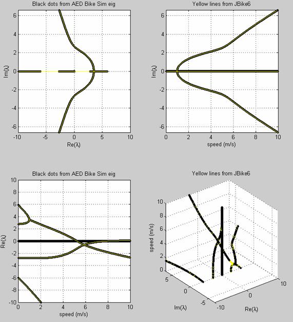
Eigenvalues from linearized equations
Eigenvalues from non-linear equations
The advent of cheap and plentiful computer power and
numerical methods provides the opportunity to simulate bicycle motion from
fully non-linear equations. Although systematic methods exist for generating
these equations that avoid the complex assumptions and simplification required
for linearized equations, the question of their accuracy remains.
Fortunately, a way exists to confirm fully non-linear equations: comparison with a known benchmark’s eigenvalues. They are intrinsic to the modeled system and are completely independent of coordinates and units chosen.
JBike6 provides these eigenvalues from its linearized equations. Here we show how to extract them from the non-linear equations, and compare the results.
In both cases the bicycle model consists of:
· 4 rigid bodies in 3 dimensions all with left-right mass symmetry.
· Connected by 3 revolute or pin joints: steering axis and two wheel hubs.
· Rider is rigidly attached to the frame (optional front and rear racks also rigidly attached).
· No friction at any joint.
· Wheels are knife-edged disks with left-right mass symmetry and polar mass symmetry, and they roll without slip or loss due to friction.
· Ground is a rigid, flat, horizontal surface.
· Only external forces are gravity, the ground reaction.
· Always starts in an upright, straight ahead configuration with some given forward velocity.
· Two non-holonomic constraints, one at each wheel contact point.
· Wheelbase: distance between wheel-ground contact points.
·
Steering axis tilt: amount steering axis is tilted from the vertical.
· Trial: distance from front wheel ground contact point to point where steering axis intersects the ground.
·
Rake: amount fork is offset, usually forward in order to reduce trail.
(Redundant and not used, but included for completeness.)
Only three coordinates are necessary to specify a bicycle on a plane:
·
Lean angle
·
Steer angle
·
Forward position of rear wheel.
However, the acceleration is taken to be zero to the
first order and so the forward velocity is constant. This leaves only two non-trivial
degrees of freedom: lean and steer angle. Two coupled second-order ordinary
differential equations represent the motion of the system.[2]
In the actual derivation for his Masters
Thesis, Scott Hand used constrained Lagrange equations and then eliminated
the constraints.
![]()
![]()
where[3]
·
![]() is the lean angle of
the rear assembly
is the lean angle of
the rear assembly
·
![]() is the steer angle of
the front assembly relative to the rear assembly
is the steer angle of
the front assembly relative to the rear assembly
· Mθ and Mψ are moments (torques) applied at the rear assembly and the steering axis, respectively, and which are both taken to be zero.
The four rigid bodies used to model a bicycle (the same as for the linearized model) with the mass and inertia of the rear rack combined with that of the rear frame and the mass and inertia of the front basket combined with that of the front fork.

The Euler Angles used to keep track of body orientation are φ, θ, and ψ:
The Coordinates are:
4 bodies in 3-D:
4 x 3 = 12 position coordinates
4 x 3 = 12 orientation coordinates (angles)
24 total coordinates
3 revolute joints:
3 x 3 = 9 position coincident constraints
3 x 2 = 6 axis parallel constraints
2 ground contact points:
2 x 1 = 2 position constraints (vertical contact)
2 x 2 = 4 non-holonomic velocity constraints (wheels roll without slip)
17 coordinate constraints and 4 velocity constraints
![]() where
where
![]() is the 3-D position
vector of body i in space-fixed
coordinates: (xi, yi, zi)
is the 3-D position
vector of body i in space-fixed
coordinates: (xi, yi, zi)
![]() is the orientation
vector of body i in space-fixed Euler
angles: (
is the orientation
vector of body i in space-fixed Euler
angles: (![]() )
)
![]() is the 3-D velocity
vector of body i in space-fixed
coordinates
is the 3-D velocity
vector of body i in space-fixed
coordinates
![]() is the angular
velocity vector of body i in
body-fixed coordinates
is the angular
velocity vector of body i in
body-fixed coordinates
The Constrained Equations of Motion are:
where D is the 'Jacobian' of the velocity constraints and gi are the 'convective' terms, and since I3 is used to represent the 3x3 identity, the body-fixed inertia matrix for body i is written J'i.[4]
Written in MATLAB version 6.5 from The MathWorks
With numerical integration via RK4, although integration is not used in the calculation of eigenvalues.
And adjusting positions and velocities back to 'constraint surface' after each numerical integration step:
·
Adjust positions by iterating with Coordinate Projection Method
·
Adjust velocities with Pseudo inverse in one step.
Use
in both implementations: 'Schwinn Crown'. Units are meters, kilograms, and
radians.
wheelbase =
1.01600000;
head_angle =
1.23879599;
trail =
0.09096800;
% rear wheel
Drearwheel =
0.68580000;
mrearwheel =
1.81818200;
Irearwheel =
[0.08551300 0.08551300 0.17102600];
alphaIrearwheel
= 0.00000000;
% front wheel
Dfrontwheel =
0.68580000;
mfrontwheel =
1.81818200;
Ifrontwheel =
[0.08551300 0.08551300 0.17102600];
alphaIfrontwheel
= 0.00000000;
% rider
mrider =
80.00000000;
xcmrider =
0.30000000;
ycmrider =
1.20000000;
Irider =
[10.53112900 2.46887100 12.00000000];
alphaIrider =
-0.25957299;
% frame
mframe =
2.50000000;
xcmframe =
0.30000000;
ycmframe =
0.50000000;
Iframe =
[0.05857900 0.34142100 0.40000000];
alphaIframe =
0.39269899;
% front fork
mfork =
1.50000000;
ucmfork =
0.00000000;
vcmfork =
0.68580000;
Ifork =
[0.05879000 0.00058800 0.05879000];
alphaIfork =
0.33200000;
% front
basket
mbasket =
1.50000000;
ucmbasket =
0.15000000;
vcmbasket =
0.80000000;
Ibasket = [0.01000000
0.01000000 0.01000000];
alphaIbasket
= 0.00000000;
% rear rack
mrack =
2.00000000;
xcmrack =
-0.10000000;
ycmrack =
0.80000000;
Irack =
[0.02000000 0.02000000 0.02000000];
alphaIrack =
0.00000000;
Rewrite the equations of
motion in matrix form:

where M is the mass matrix, C is the damping matrix, K is the stiffness matrix, and D is the differential operator. Note that for the upright bike Cθθ = 0, and so it did not appear above in the equations of motion.
Combine
the M, C, and K matrices into 2
4x4 matrices, A and B,
 and
and 
and
calculate the 4 generalized eigenvalues
of them via:
Ax = λBx
Where
the values of λ that satisfy the
equation are the generalized eigenvalues and the corresponding values of x are the generalized right
eigenvectors.
In MATLAB:
B = [M zeros(2); zeros(2) eye(2)];
A = [-C -K; eye(2) zeros(2)];
[V,D] = eig(A, B);[5]
Screen shot of JBike6 program showing the bicycle parameters,
a stylized drawing of the bicycle, and the calculated eigenvalues for a range
of forward speeds.

Represent the system in
state-space form as
![]()
and assume a solution of the form ![]() .
.
Then the eigenvalues, λ, of the matrix [A] describe stability: stable for λ < 0, unstable otherwise.
To construct this matrix [A] for a nonlinear system being solved numerically, recognize that the
function to compute the accelerations (called by the ode solver, RK4 in this
case) has the form ![]() .[6]
.[6]
Thus the matrix we seek is
merely  .
.
However, ![]() is not some function
that we can simply differentiate symbolically.
is not some function
that we can simply differentiate symbolically.
Instead, to calculate
partial derivatives numerically, use the definition of the derivative:
![]() (for forward
differencing, with error O(ε))
(for forward
differencing, with error O(ε))
![]() (or even better:
centered differencing, with error O(ε2))
(or even better:
centered differencing, with error O(ε2))
If access to calculated accelerations is available
(which in this case is the output of the function called by the ode solver)
then
![]()
In order to select the best
value for epsilon, we simply iterate until convergence.
The value of epsilon for each state variable and forward speed is chosen in a loop in which it is decimated until the resulting candidate values for a column in the matrix converge. The best value turns out to be 1e-11.
The eigenvalues of this matrix [A] can be compared to the eigenvalues from the linearized equations. In this particular case, because the non-linear equations use 48 state variables instead of the 4 used in the linearized equations to represent the 2 non-trivial degrees of freedom in the system, 48 values are generated. 4 of them correspond to the 2 non-trivial degrees of freedom in the system, and can be compared to the 4 generated from the linearized equations.
In MATLAB:
v0 = v0_min; % start with the first forward
speed
speed = 1; % index this as number 1
while v0 <= v0_max % while there are more forward speeds
to use
for sv = 1: state_variables % for
each state variable
e = zeros(state_variables, 1); %
initialize an epsilon vector
e(sv, 1) = epsilon; %
set one value to non-zero
for direction = -1:2:1 %
for each dir for center diff
z(:, n) = z_0 + (epsilon .* direction);
% add epsilon to st v
% Apply constraints to the four bodies
% iterate to adjust current
positions subject to constraints
% adjust current velocities
subject to constraints
% Calculate accelerations (Left Hand Side)/(Right Hand Side)
[z(:, n+1), lambdas(:, n+1)] = ode(z(:, n), M, Mo_b, f, r_b);
if direction == -1
f_z_0_m_e = z(:, n+1); % f(z_0 –
epsilon)
else
f_z_0_p_e = z(:, n+1); % f(z_0 +
epsilon)
A(:, sv) = (f_z_0_p_e - f_z_0_m_e) / (2 * epsilon); % add
end
end
end
[V,D] = eig(A); %
calculate eigenvalues
eigs(:, speed) = diag(D); % store them away
v0s(speed) = v0; % store
forward speed
v0 = v0 + v0_step; %
increment forward speed
speed = speed + 1; %
increment index
end
The plots below show the excellent match of both real and imaginary parts of eigenvalues from the two methods.
The plots below show the
difference between just the real parts
of the values from the two methods.
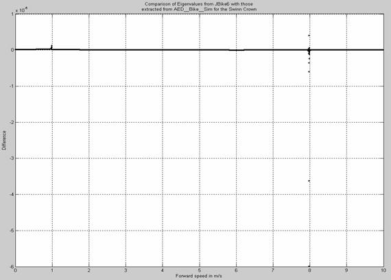
at 10-6
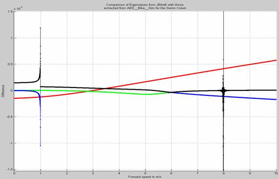
at 10-7

at 10-8
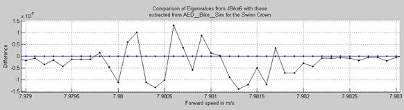
at 10-5 and only the part of the forward speed range near the
capsize speed.
Maximum difference between the two methods occurs near the capsize speed (7.9807 m/s), where an eigenvalue crosses the real axis from negative to positive. The difference peaks at just under 1.5e-05.
Another, smaller increase in error occurs just before (forward speeds < 1 m/s) a double root: a bifurcation where two eigenvalues with different real parts and zero imaginary parts approach the same value and then (for higher forward speeds) have the same real parts and complimentary imaginary parts. There the difference peaks at just over 1e-07.
In all other cases, the difference between eigenvalues from the two different methods remains less than 6e-08.
The non-linear equations of motion are confirmed.
Investigate and eliminate spike in difference between eigenvalues from linearized and non-linear equations when velocity is near 8 m/s.
Investigate generating more accurate eigenvalues from non-linear model with more accurate derivatives.
Andy Ruina, Professor of Theoretical
and Applied Mechanics at
Arend Schwab, Assistant Professor in Applied Mechanics at of Delft University of Technology and creator of TAM 674: Applied Multibody Dynamics, the class in which we derived the non-linear bicycle model and implemented it in MATLAB. Also co-author of JBike6.
Jim Papadopoulos, author of JBike5 and co-author of JBike6
The rest of the Theoretical
& Applied Mechanics Biorobotics and Locomotion Lab at
Fellow T & AM graduate student Geoff Recktenwald.
Here are some video clips of the animated simulation confirmed by JBike6.