JBike6
Help
(
JBike6 is a tool, written in MATLAB, you can use to calculate and examine the eigenvalues (i.e., perturbation-growth exponents) for an idealized, uncontrolled bike.
It uses physical parameters (pre-defined or user-entered) to describe a particular bike, then calculates and plots the linearized perturbation-growth eigenvalues over a range of forward speeds that you specify.
An idealized, rigid, uncontrolled bike with rigid rider has four eigenvalues: either all real (non-oscillatory); two real plus a complex pair representing oscillatory motion; or in rare cases two complex pairs. (Idealized means that the bodies are perfectly rigid and symmetrical about the midplane, the joints are frictionless, and it rolls on knife-edge wheels without loss due to friction and without slipping on a smooth, rigid, horizontal plane.)
In general, a bike design is self-stable at those forward speeds for which the real parts of all the eigenvalues are less than zero. (Self-stable means that without external input, it will eventually roll straight and upright even if perturbed.) Such behavior can easily be seen in real-world bicycles, when rolled without a rider. Follow this link for more details and a video.
For brief help just see the ‘Parameters’ section from this help file.
Contents (all links to items on this page)
Installing
Download the distribution file onto your computer.
Unzip the distribution file into a subdirectory on your computer.
Running
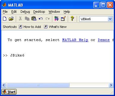 Start
MATLAB from The Mathworks. The JBike6 GUI
(Graphical User Interface) requires MATLAB version 6.0 or higher. To run
without the GUI see the section below on Running JBike6 without the GUI.
Start
MATLAB from The Mathworks. The JBike6 GUI
(Graphical User Interface) requires MATLAB version 6.0 or higher. To run
without the GUI see the section below on Running JBike6 without the GUI.
Tell MATLAB where to find JBike6 by either:
1. In MATLAB, make the current directory the directory into which you unzipped JBike6. You can do this through the MATLAB desktop or with the cd command in the MATLAB command window.
2. Alternatively, if you have MATLAB version 7.0 or higher, you may add the JBike6 directory to the MATLAB path. You can do this through the ‘Set Path…’ option of the ‘File’ menu or with the path command in the MATLAB command window.
Run the file JBike6.m by either:
1. typing ‘JBike6’ on the MATLAB command line and pressing the ‘Enter’ key on your keyboard, or
2. opening the JBike6.m file in MATLAB’s Editor and selecting ‘Run’ from the ‘Debug’ menu or pressing the ‘F5’ key.
In fact, if you run JBike6 from MATLAB’s Editor, you may skip telling MATLAB where to find JBike6, and it will prompt you to let it automatically either change the current directory or add to the path.
See the MATLAB help for more details.
Running without the GUI
If there is some functionality you need that the GUI (Graphical User Interface) does not offer, or if the GUI is getting in your way, you can run JBike6 as a command-line application. The first thing you need to do to make this possible is edit the JBike6.m file and change the line that reads:
use_GUI
= 1
to
use_GUI
= 0
Then simply run JBike6 as before, and now it will not launching the GUI. JBike6 reads from the JBini.m file all the parameters that you would specify in the GUI.
The JBini.m file contains comments to explain the variables, their coordinate systems, and their units. When you run JBike6 without the GUI, it draws the same bike diagram and eigenvalue plot as with the GUI, but in separate windows.
For more details about running JBike6 without the GUI, see the Appendix below.
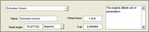 You
can specify the mass, location, orientation, and inertia for all the bodies
that make up a bike, or you can load a previously saved parameter set from
the pull-down menu in the upper left of the window.
You
can specify the mass, location, orientation, and inertia for all the bodies
that make up a bike, or you can load a previously saved parameter set from
the pull-down menu in the upper left of the window.
You can save all the parameters that describe a particular bike configuration and retrieve them for later use. You may also simply discard them if they do not prove interesting or useful.
Selecting an existing bike design
To select an existing bike design, provided with JBike6 or previously saved by you, simply select one from the pull-down list in the upper-left corner of the main window.
JBike6 will display all of its parameters, draw a stylized diagram of it, and calculate its eigenvalues and plot them.
Calculating and plotting eigenvalues
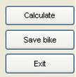 To
calculate and plot the eigenvalues for a bike, click on the ‘Calculate’ button in the upper right of the window. Jbike6 reads
all the current bike parameters you have
specified, checks them for validity, draws the bike, calculates the eigenvalues, and plots
them.
To
calculate and plot the eigenvalues for a bike, click on the ‘Calculate’ button in the upper right of the window. Jbike6 reads
all the current bike parameters you have
specified, checks them for validity, draws the bike, calculates the eigenvalues, and plots
them.
There is an option in the ‘Settings’ menu to turn on and off the display of status messages in MATLAB’s command window while calculating eigenvalues. Turn this on to see what JBike6 is doing while you wait. Turn this off to save a little time during each calculation.
Specifying a new bike design
There are two ways that you can specify a new bike design:
1. Start from scratch: select ‘Blank’ from the pull-down list of bikes. All the parameter values are zero. Type a new name and all the parameter values that you want. Then save the new design. JBike6 cannot work with a design you enter from scratch until you save it.
2. Start with an existing design: select any pre-existing design from the pull-down list of bikes. Type a new name and change all the parameter values that you want.
Each number may contain any of the digits 0 through 9, a decimal point, a leading + or - sign, and an 'e' or 'd' preceding a power of 10 scale factor: for example the ASCII text string ‘-1.23e2’ represents the value -123. Read more about precision below.
Until you press the 'calculate' button, all the text-entry controls, such as ‘trail’ and ‘mass’ contain whatever and exactly what you type in there. As soon as you press the 'calculate' button, or otherwise start JBike6 on the task of calculating and plotting the eigenvalues, it reads the contents of each control and uses MATLABs internal ‘str2num’ function to convert it to a an IEEE 64 bit floating point number. That function returns a number if it can, otherwise it returns nothing: the ‘length’ of the variable contents is actually zero.
The calculations required to generate eigenvalues cannot work with variables that contain nothing, and they would report an error if they did, so JBike6 checks for this condition, and when it occurs, sets the value to the 64 bit representation of zero. Then, for completeness, it puts back into that control the ASCII text string representation of that number. So, any field that did not have a valid number, including fields that were blank, get set to '0'.
Saving bike parameters
You can save all the parameters of a particular bike design either with the ‘Save bike’ button, the ‘Save bike parameters’ option of the ‘File’ menu, or by pressing CTRL-S (the ‘Control’ key and the ‘s’ key simultaneously).
When you select ‘Save bike‘, JBike6 writes an ASCII text configuration file that contains all the parameters necessary to describe the bike. The file name always begins with ‘BJini’, contains the bike name that you specify, and ends with an ‘.m’ extension. In order to make the file name usable by JBike6 the next time it starts, it removes periods and parenthesis and replaces blanks with underscore characters. Also to be a valid file name in the MS Windows file system it cannot contain any of the following characters: \ / : * ? ” < > |, so JBike6 removes them as well.
JBike6 also saves the current gravity constant g and calculated critical speeds in this file, if they exists, but only as comments and will not read them back in. Each time you select a different bike or select ‘Calculate’, JBike6 uses the current value of g, which you can specify, to calculate eigenvalues and the weave and capsize speeds.
When JBike6 starts, it reads all the configuration files it can find and sorts them alphabetically to build the list of available bikes for the pull-down menu. The directory from which JBike6 reads and to which it writes bike configuration files defaults to the JBini_files subdirectory of the program directory: where the JBike6 program files are located. You may change this directory by selecting ‘Set ‘save bike’ directory…’ from the ‘Settings’ menu.
Discarding bike parameters
You may discard changes you make to bike parameters if they do not prove interesting or useful. To discard them, simply select a bike (the same one or a different one) from the pull-down menu or exit JBike6.
Saving settings and styles
There is an option in the ‘Settings’ menu to save all the other settings, such as the forward speeds, the gravitational constant, etc., and styles when JBike6 exits. If you have this setting checked, JBike6 writes all your settings to a configuration file, JBconfig.m. The next time you start JBike6, it will read this file and restore all your settings and styles. Note that JBike6 can only save your settings and styles if you exit by either the ‘Exit’ option in the ‘File’ menu or the ‘Exit’ button. If you exit with the ‘close window’ button at the upper right of the window, MATLAB does not give JBike6 an opportunity to save your settings and styles.
Saving calculated eigenvalues
There is an option in the ‘File’ menu to save the calculated eigenvalues along with their corresponding speeds to a file. When you specify the file name, you can specify either a MATLAB *.mat file or an ASCII text file. After you specify the file name and type, JBike6 writes the eigenvalues and their corresponding speeds to that file in the appropriate format.
You can open a MATLAB *.mat file with the ‘load’ command at the MATLAB command prompt. See the MATLAB help for more details. You can open an ASCII text file in Notepad, Microsoft Excel, or similar application.
Exiting JBike6
There are several ways to exit JBike6:
1. Select ‘Exit’ from the ‘File’ menu.
2. Press CTRL-X (the ‘Control’ key and the ‘x’ key simultaneously).
3. Click on the ‘Exit’ button in the upper right-hand corner of the main window.
4. Click on the ‘Close Window’ button n the extreme upper right-hand corner of the main window.
5. Exit MATLAB, by any of its various methods. See the MATLAB help for more details.
Caution: if you have checked the ‘Save settings and styles when exiting’ option in the ‘Settings’ menu, and you exit JBike6 by any method other than 1, 2, or 3, above, then MATLAB does not give JBike6 an opportunity to save styles and settings. Any changes you have made to settings or styles will be lost.
You specify a particular bike configuration by entering certain parameters. For the idealized model of a bike that JBike6 uses, the parameters that you can enter on the main window provide all the information that JBike6 needs to calculate the eigenvalues.
All mass is in kilograms, distance in meters, and speed in meters per second.
You may toggle between angles in degrees or radians by selecting either one from the pull-down menu next to the head angle. JBike6 automatically recalculates the values of all the angle parameters to match the units you choose.
JBike6 treats all parameters as decimal expansions to 16 significant digits. In other words, 72 degrees really means 72.00000000000000 degrees, even though trailing zeros are not shown. Read more about precision below.
The parameters you enter can not be arbitrary. As described below, certain ones have to be nonzero or positive. In order for the model to make physical sense, you have to limit certain ones: keep the mass above the ground, keep wheels from bumping each other, etc.
When JBike6 displays values in its own window, it may truncate some, such as the critical speeds displayed above the eigenvalue plot, in order to fit in the available space, but it displays values in the MATLAB command window with all 16 available digits. Read more about precision below.
JBike6 displays ‘tooltips’ when you hover the cursor over any of the parameter input controls.
Bike Parameters
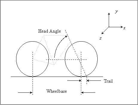
The wheelbase is the horizontal distance between the hub (or ground contact point) of the front wheel and the rear wheel. The wheelbase can be positive or negative, but not zero, and the magnitude should be greater than sum of wheel radii in order for bike to be physically possible.
The head angle is the angle the head tube (steering axis) makes with the horizontal. A 90° head angle would be vertical. By convention, positive angles are clockwise from the horizontal. Common head angles for road bikes range from 70° to 75°. JBike6 accepts any angle, but angles close to 0° are not practical for steering.
The trail is the horizontal distance from the front hub (or ground contact point) to the point where the steering axis intersects the ground. By convention, positive trail is when the front wheel contact point is behind, toward the rear wheel, the steering axis intersect point.
Component Parameters
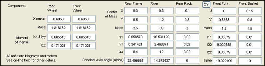
Rear: The center of mass of the rider, rear frame, and rear rack are all measured in the xy-coordinate system. The origin is located at the rear wheel contact point, the x-axis is horizontal forward, the y-axis is vertical up, and the z-axis is out of the plane following the right-hand rule.
The wheelbase and wheel diameters completely specify the locations of the wheel centers of mass.
![]() Front: You can specify the center of
mass of the front fork and the front basket in either the uv-coordinate system or the same xy-coordinate system as the rear
of the bike. You can toggle between these two coordinate systems by clicking on
the XY or UV button at the upper left of the front fork parameters. The labels
below the button indicate which coordinate system JBike6 is currently using.
The origin of the uv-coordinate system is located at the intersection of the
steer axis with the ground and the coordinate system is rotated so that the v-axis is along the steering axis:
rotated from the y-axis counter clock-wise by π/2
radians (90°) minus the head angle. (See the
bike diagram below.) JBike6 automatically recalculates the values of front
fork and basket coordinates to match the coordinate system you choose. JBike6
uses the uv-coordinate system internally, and saves (and reads) bike configurations
with the uv-coordinate system.
Front: You can specify the center of
mass of the front fork and the front basket in either the uv-coordinate system or the same xy-coordinate system as the rear
of the bike. You can toggle between these two coordinate systems by clicking on
the XY or UV button at the upper left of the front fork parameters. The labels
below the button indicate which coordinate system JBike6 is currently using.
The origin of the uv-coordinate system is located at the intersection of the
steer axis with the ground and the coordinate system is rotated so that the v-axis is along the steering axis:
rotated from the y-axis counter clock-wise by π/2
radians (90°) minus the head angle. (See the
bike diagram below.) JBike6 automatically recalculates the values of front
fork and basket coordinates to match the coordinate system you choose. JBike6
uses the uv-coordinate system internally, and saves (and reads) bike configurations
with the uv-coordinate system.
For the inertia tensor of each mass, the 1-axis is rotated counter-clock-wise from the horizontal by the principal axis angle (alpha) for that mass, and the 2-axis is rotated in the same direction from the vertical by the same amount. (See the bike diagram below.) The principal axis angle for the front fork and the front basket is always measured counter clock-wise from the axes of the xy-coordinate system, even if their center of mass is specified in the uv coordinate system. For further discussion of inertia tensors, see the More on Inertia Tensors section in the appendix below.
I11 represents the inertia about the 1-axis, I22 the inertia about the 2-axis, and Izz, about the z-axis.
Note that the wheels are treated as symmetrical about the z-axis, and so Ixx = Iyy.
Before JBIke6 begins calculating eigenvalues, it combines the rear frame, rider, and rear rack into one single rigid body, and it combines the front fork and front basket into a second single rigid body. This is necessary because of the simplified bike model used to derive the equations of motion that JBike6 uses.
For further discussion see the More on Parameters section in the appendix below.
Forward Speeds
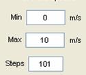 The
actual forward speed of the bike is a crucial component of the eigenvalue calculations. In order
to see how eigenvalues change with speed, you can enter a range of speeds to
use. You can specify a minimum and maximum speed, and the number of individual
speeds (steps) to use in between.
The
actual forward speed of the bike is a crucial component of the eigenvalue calculations. In order
to see how eigenvalues change with speed, you can enter a range of speeds to
use. You can specify a minimum and maximum speed, and the number of individual
speeds (steps) to use in between.
Gravity
![]() You
can change the gravitational acceleration constant (small ‘g’) used in the
calculations by selecting the ‘Set gravity constant…’ option of the ‘Settings’
menu. For your convenience, the currently set value of g is displayed at the bottom
of the window. You may enter any positive value for gravity that you want.
JBike6 will calculate different weave and capsize
speeds for different values of g.
You
can change the gravitational acceleration constant (small ‘g’) used in the
calculations by selecting the ‘Set gravity constant…’ option of the ‘Settings’
menu. For your convenience, the currently set value of g is displayed at the bottom
of the window. You may enter any positive value for gravity that you want.
JBike6 will calculate different weave and capsize
speeds for different values of g.
It can be shown that vastly different values (for example, g on the moon) drastically change the zero-speed eigenvalues; but at high speed only the capsize eigenvalue (value: nearly zero) is noticeably affected. In other words, high speed bike dynamics are largely independent of gravity.
Read more about Gravity in the Appendix below.
Precision
In general, you can treat all inputs as having 16 significant digits. It does not matter whether you enter 3, 3.0, or 3.00000000000000. JBike6 stores all of them the same way internally.
A change near the 7th digit of the trail parameter produces a change near the 7th digit of the calculated weave speed, a change near the 8th digit produces a change near the 8th digit, and the 9th to the 9th, etc.
Finally, the comparison used to verify the results from JBike6 is able to match 14 digits of the values that JBike6 produces with those from other methods.
Read more about Precision in the Appendix below.
Parameter Limitations
Wheelbase: can be positive or negative, but not zero, and magnitude should be greater than sum of wheel radii in order for bike to be physically possible.
Head angle: any angle, but angles close to 0° are not practical for steering. JBike6 produces identical results for values ±360, when using the uv-coordinate system, and ±180 when using the xy-coordinate system.
Trail: any value†
Wheel diameters: must be positive.*
Mass: must be greater than or equal to zero. When the ratio between masses approaches 1e20, the determinant of the mass matrix becomes zero, and JBike6 is unable to continue.
Inertia: each value must be greater than or equal to zero and I11 + I22 ≥ Izz, Izz + I11 ≥ I22, and I22 + Izz ≥ I11.
Principal Axis Angles: any value.†
Speeds: any values, including negative, so long as min and max are not the same.
Speed steps: at least 2, or 3 in order to find double root speeds via interpolation method.
Gravity: must be greater than zero.*
See Appendix for additional guidelines.
* greater than zero actually means the smallest positive value, 4.9407e-324, or greater.
† You may use scientific notation, with the letter e to specify a power-of-ten scale factor, and a maximum of 16 digits of precision, to enter values: 1e1 = 10. The smallest magnitude is 4.9407e-324, and the largest is 1.7976e+308
Errors
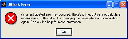 JBike6
does check all the parameters you enter to make sure that all the requirements
listed above are met. Never-the-less, there may be unforeseen parameter
combinations for which JBike6 or the underlying MATLAB are unable to calculate
the eigenvalues. For example, the determinant of the mass matrix is zero. In
that case JBike6 will report an error, as seen to the right. You may simply
change the parameters and try to calculate the eigenvalues again.
JBike6
does check all the parameters you enter to make sure that all the requirements
listed above are met. Never-the-less, there may be unforeseen parameter
combinations for which JBike6 or the underlying MATLAB are unable to calculate
the eigenvalues. For example, the determinant of the mass matrix is zero. In
that case JBike6 will report an error, as seen to the right. You may simply
change the parameters and try to calculate the eigenvalues again.
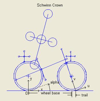
JBike6 draws a representation of the bike you specify in the lower left half of the window. It draws the ground plane, the steering axis as a dotted line, and stylized representations of the wheels, frame, fork, rider, rear rack, and front basket.
It uses stylized dumbbells to illustrate the inertia parameters of each body. You can think any mass you specify as being divided into 6 equal-mass disks (represented by circles, only 5 of which are visible in 2D) located on the ends of three mutually-orthogonal dumbbell arms, oriented along the principal inertia axes. The size of the circles represents the mass with a radius of
![]() .
.
The length of the arms represents how far the mass is distributed from the center of gravity. Each body has its own Principal Axis angle (alpha) to specify how the I11 axis is rotated (counter clock-wise) from the always-horizontal x axis.
The farther away the disks are from the center along the 1-axis and the 2-axis, the more inertia the object has about the z-axis. The larger the value of any one of the three, up to the limits described above, the farther away the disks will be along the other two axes.
The depth of the wheel rims represents the distribution of the wheel mass away from the center of gravity. The deeper the rim, the more inertia the wheel has about the z-axis: its hub. The outer circle is at the actual rim diameter that you specify. The inner circle is at a radius of
![]() .
.
Note, it is OK to have a body with large inertia and small mass – even though the dumbbell is drawn as penetrating the ground. It could, in fact, be due to a very tall, lightweight pole extending upward, plus a large mass extending only slightly downward.
See appendix for further explanation.
In the ‘Settings’ menu, you can toggle on or off the display of the coordinate axes and labels in the bike diagram.
 After
calculating the eigenvalues for each forward speed, JBike6 plots the real
component of them against the forward speed in the lower right half of the
window with dots.
After
calculating the eigenvalues for each forward speed, JBike6 plots the real
component of them against the forward speed in the lower right half of the
window with dots.
Critical Speeds
In addition simply calculating and plotting the eigenvalues for a range of forward speeds, JBike6 calculates some critical speeds at which the bike behavior undergoes a qualitative change.
JBike6 can also display and label these values in the MATLAB command window.
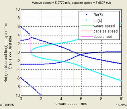
Weave Speed
The forward speed at which oscillatory motion neither grows nor decays. This is represented on the plot by a vertical line. Oscillatory motion is that motion in which the bike leans and steers back and forth.
At speeds below this weave speed, the oscillations will grow until the bike falls over. There may not be a weave speed for a particular bike configuration.
Weave is a sinuous motion of the bike, steering and leaning left and right. When it leans left it also steers left, more than enough to simply return to the upright. The oscillation magnitude is steady at the weave speed, and grows below or shrinks above.
A conventional bike has a single nonzero speed interval of stability, and the weave speed is the lower boundary of this interval. Thus an uncontrolled bike that slows just below the weave speed becomes unstable by weaving. But, if the weave speed is above the capsize speed, there probably is no stable interval.
Capsize Speed
The forward speed at which capsize motion neither grows nor decays. This is represented on the plot by a vertical line. Capsize motion is that motion in which the bike slowly leans and steers, without oscillation, farther and farther until it falls over.
At speeds above this capsize speed, the capsize motion will progress until the bike falls over. There may not be a capsize speed for a particular bike configuration. Odd designs have been found which have no finite capsize speed, and are stable at all speeds above the weave speed.
In capsize, the bike leans and steers to the same side, but the steer is never sufficient to balance or correct the lean. At the capsize speed it just travels in a circle without uprighting. Above the capsize speed, it spirals tighter and tighter (leaning and steering more and more.) Capsize generally takes many seconds until full collapse.
For more information on eigenvalues, stability, and how to interpret this plot see the sections of eigenvalues and interpretation of results below.
Stable Region
For emphasis, JBike6 can shade the region between the weave speed and the capsize speed. You can turn on and off this shading with the ‘Shade stable region’ option of the ‘Settings’ menu and set the color used with the ‘Stable region shade color…’ option of the ‘Plot Styles’ menu. If there is a weave speed but not a capsize speed, JBike6 shades the region from the weave speed to the highest forward speed you specify.
Double Root Speeds
The speeds at which double roots occur, where two real roots start forming a complex conjugate pair of roots or vice versa, are marked by vertical lines. This is where oscillatory behavior begins, at a frequency that grows rapidly as the speed is surpassed.
JBike6 offers two methods for finding these roots:
1. analytical: using analytical manipulations supplemented by polynomial root finding. This can take several minutes.
2. interpolation: by interpolating from the calculated eigenvalues. This can take several seconds.
There is an option for you to select which method to use and an option to toggle this functionality on and off .in the ‘Settings’ menu.
There is an option in the ‘Settings’ menu to toggle on and off the display of the imaginary components of the eigenvalues. This can be useful in understanding the frequency of the oscillatory motion.
Note that changes you make in the ‘Settings’ menu do not take effect until you calculate and draw the eigenvalues again.
Calculated Stability
To aid in comparing particular bike designs, JBike6 calculates and displays the ‘maximum stability’, the forward speed at which it is found, and the ‘total stability’.
‘Maximum stability’ is exactly and only the value of the least negative calculated eigenvalue and the forward speed at which is was found.
‘Total stability’ is merely the sum of the least negative calculated eigenvalues multiplied by 10 times the size of the speed steps.
Note that both of these values are only found from the eigenvalues actually calculated at the forward speeds you specify. Also, these values only refer to the self-stability of a completely uncontrolled bike, as specified in the model, and may have no bearing on the actual handling characteristics experienced by a rider.
Finally, JBike6 calculates the tipping moment of all the masses about the front wheel. If this value is positive, a real bike with masses distributed as specified would tip forward, JBike6 displays a warning message in the command window and at the bottom of the bike diagram.
 Plot Styles
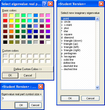
You can change the colors, sizes, symbol types, and line types that JBike6 uses to plot the eigenvalues and critical speeds. Select the appropriate option from the ‘Plot Styles’ menu and then pick the color, enter the size, or pick the symbol or line type you want. You can even set the plot background color.
You can also select ‘Black and white styles’ to use a predefined set of black and white colors and appropriately differentiated set of symbol types and line types suitable for black and white output.
You can quickly increase or decrease the sizes of all the plot styles with the ‘Enlarge all eigenvalue plot styles’ and ‘Shrink all eigenvalue plot styles’ menu options respectively.
Finally, you can select ‘Reset default colors’ to return the plot windows to the original colors, sizes, symbol types and line types.
There is an option in the ‘Settings’ menu to toggle on and off the display of a legend. You may click on and move the legend from its default position if necessary. There is also a context menu with style options that you can access by right-clicking on the legend. See the MATLAB help for further information about manipulating a legend.
Note that changes in the ‘Plot Styles’ menu do not take effect until you calculate and draw the eigenvalues again.
Additional eigenvalue plots
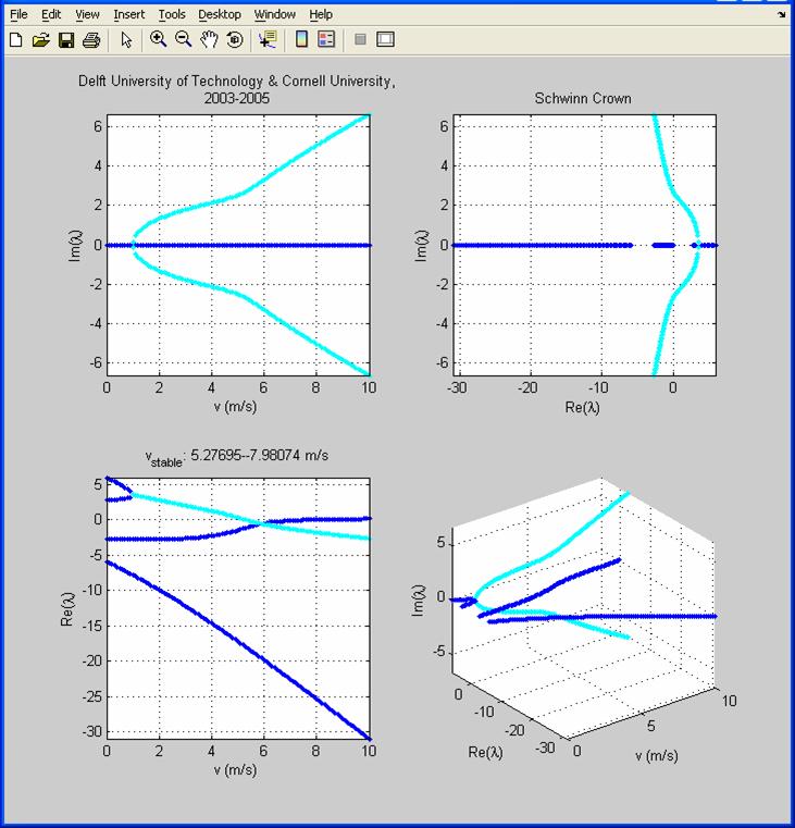
There is also an option in the ‘Settings’ menu and a check box next to the eigenvalue plot to toggle on and off the display of an additional window with four different plots:
1. V vs Re(λ): Forward speed verses the real parts of the eigenvalues
2. V vs Im(λ): Forward speed verses the imaginary parts of the eigenvalues
3. Re(λ) vs Im(λ): The real parts of the eigenvalues verses the imaginary parts of the eigenvalues
4. V vs Re(λ) vs Im(λ) in 3D.: Forward speed vs the real parts of the eigenvalues verses the imaginary parts of the eigenvalues
You can use the MATLAB magnify, pan, and rotate tools on these plots along with the rest of MATLAB’s plot manipulation tools. See the MATLAB help for more details.
In the 3D plot, the imaginary eigenvalue components (representing oscillation frequency) are plotted more conventionally: perpendicular to the real eigenvalue components.
There is an option in the ‘Settings’ menu to use the styles from the single plot in the main window in these 4 plots additional plots. Select the ‘Use Styles menu styles in additional plots’ to have JBike6 draw the real and imaginary parts of the eigenvalues with the styles you have specified in the ‘Plot Styles’ menu.
JBike6 applies colors to the real and imaginary parts slightly differently than in the single eigenvalue plot in the main window.
· In the single eigenvalue plot in the main window, JBike6 plots the real components of all the eigenvalues in one color, and, if you have the ‘Draw imaginary parts of eigenvalues’ option checked in the ‘Settings’ menu, the imaginary components in a different color on the same axis.
· In the additional, four-plot window, JBike6 always plots real and imaginary components on different axis. It also, if you have the ‘Use Styles menu styles in additional plots’ option checked in the ‘Settings’ menu, uses the ‘real’ color only when an eigenvalue does not have an imaginary component, and it plots all complex eigenvalues with the ‘imaginary’ color.
 MATLAB
Command Window Values
MATLAB
Command Window Values
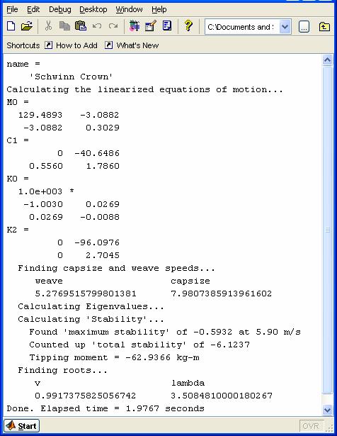
As JBike6 calculates certain values, weave speed and capsize speed for example, it can also display these, to all possible 16 digits, in the MATLAB command window.
This can slightly slow the entire operation, and so there is an option in the ‘Settings’ menu to turn this display off an on.
The full list of values displayed includes:
The bike name
The mass matrix: M0
The damping matrix: C1
The stiffness matrix, in two pieces
that are added together before calculating eigenvalues: K0 and
The calculated ‘maximum stability’, ‘total stability’, and tipping moment.
The eigenvalues and speeds at which double roots appear
The elapsed time
You can plug the values from the mass, damping, and stiffness matrices into the equations of motion given below to perform further analysis such as integrating them forward in time to evaluate lean and heading due to steering input.
Background and Theory
A bike is a non-holonomic system because of how its wheels interact with the ground: its configuration is path-dependent. In order to know its exact configuration, especially location, it is necessary to know not only the configuration of its parts, but also their histories: how they moved over time. This complicates mathematical analysis.
A bike is also an example of an inverted pendulum. Thus, just as a broomstick is easier to balance than a pencil, tall bikes can be easier to balance than short ones because their characteristic time of falling is longer.
The idealized model of a bike used by JBike6 is a conservative system: there is no energy dissipation. At forward speeds for which weave oscillations decrease with time, the energy is being converted from the weave into an increase in the forward speed. Although it is conservative, it is not Hamiltonian due to the non-holonomic constraints mentioned above.
Finally, in the language of control theory, a bike exhibits non-minimum phase behavior. To turn to the right, you must initially turn to the left and visa versa.
The model
JBike6 uses an idealized rigid-body dynamics model of the bike, defined as four interconnected rigid bodies interacting with a horizontal ground plane:
1. A rear wheel with left-right mass symmetry and polar mass symmetry, rolling on a knife edge, and revolutely connected to the rear frame.
2. A rear-frame, rider, rear rack, all in one rigid assembly, with left-right mass symmetry, revolutely connected to the front fork. (Although JBike6 uses only the entire assembly’s mass and inertia, you may separately define a frame, rider, and rack in case you have data only for the separate sub-components.)
3. A front-fork, handlebar, and front basket, all in one rigid assembly, with left-right mass symmetry, revolutely connected to the front wheel.
4. A front wheel with left-right mass symmetry and polar mass symmetry, rolling on a knife edge.
In the complete bike assembly, when held upright and steered straight, all components share the same symmetry midplane. The wheel axles are normal to that plane and the steer axis is in that plane.
All the revolute joints are frictionless, and the rolling occurs without dissipation or slippage.
There is no propulsive or braking torque, and no slope or air resistance.
JBike6 uses a linearized analysis for small deviations from the upright straight condition. You should expect perfect accuracy only when steer and lean angles are infinitesimal, however you may expect that many results and trends [easy to find because the governing equations are linear] also hold quite well for realistically large angles. Determining the inaccuracy resulting from realistic angles is the province of nonlinear analysis.
Note that in a linearized analysis near the upright straight condition, the bike’s full geometry and mass distribution is not needed – for example, there is no ‘pitch’ motion of the rear frame assembly, so that component of inertia is irrelevant. Also, apart from establishing the rotation rate of the wheels, wheel diameter is unimportant – one could as easily envision ‘infinitesimal’ wheels placed at the bike’s two contact points. JBike6 takes full data as input so that they can be unambiguously available for nonlinear analysis.
The two degrees of freedom are q=[lean angle, steer angle], with lean to the right (clock-wise when viewed from the rear) and steer to the left (counter-clock-wise when viewed from above) is positive when driving forward.
Eigenvalues
Definition
Eigenvalues are defined, as the scalar quantities λ
such that for matrix [A], if there is a non-zero vector ![]() for which this
equation [A]
for which this
equation [A]![]() = λ
= λ![]() is true, then
is true, then ![]() is an
eigenvector of [A] and λ is its corresponding eigenvalue. Another way to
think of them is that if the matrix [A] is a transformation, then the
eigenvectors of [A] are those vectors whose directions are not changed
by that transformation, and the corresponding eigenvalues are how much the magnitudes
or lengths of those eigenvectors are changed.
is an
eigenvector of [A] and λ is its corresponding eigenvalue. Another way to
think of them is that if the matrix [A] is a transformation, then the
eigenvectors of [A] are those vectors whose directions are not changed
by that transformation, and the corresponding eigenvalues are how much the magnitudes
or lengths of those eigenvectors are changed.
Read more about Eigenvalues in the Appendix below.
Interpretation
To see where eigenvalues come into play in the bike
system, represent it (see linearized equations of
motion below) in state-space form as ![]() (where
(where ![]() is a vector that
represents all the coordinates and their speeds necessary to describe the
system,
is a vector that
represents all the coordinates and their speeds necessary to describe the
system, ![]() is a vector that
represents their time derivatives: speeds and accelerations, and
is a vector that
represents their time derivatives: speeds and accelerations, and ![]() is a matrix that incorporates
is a matrix that incorporates
 all the necessary
parameters), and assume a solution to the system of differential equations to
have the form
all the necessary
parameters), and assume a solution to the system of differential equations to
have the form ![]() where λ are the
eigenvalues of the matrix
where λ are the
eigenvalues of the matrix ![]() , t is time, and e is the base of the natural logarithm.
, t is time, and e is the base of the natural logarithm.
Exponential growth or decay
Then, for any positive values of λ, ![]() > 1, the solution
> 1, the solution ![]() will grow. For
negative values of λ,
will grow. For
negative values of λ, ![]() < 1, the solution
< 1, the solution ![]() will shrink. A
growing solution moves away from the initial state and so is unstable, and a
shrinking solution returns to the initial state and so is stable.
will shrink. A
growing solution moves away from the initial state and so is unstable, and a
shrinking solution returns to the initial state and so is stable.
Thus the eigenvalues, λ, of the matrix [A] describe stability: stable for λ < 0, unstable otherwise.
Oscillatory motion
For complex
conjugate values of λ
(which are quite common, see the plot of forward speed vs the imaginary
component of the eigenvalues to the right), the solution (and hence the bike)
will exhibit oscillatory motion (this can be predicted from Euler’s equation: ![]() where
where ![]() : an imaginary number), either growing or
shrinking, depending on the sign of the real part of the eigenvalues.
: an imaginary number), either growing or
shrinking, depending on the sign of the real part of the eigenvalues.
The frequency of the oscillation is proportional to the magnitude of the complex number.
In general, during oscillation the steer and lean may be out of phase somewhat. In fact, the phase lag can be predicted by comparing the real and the complex parts of the elements of the weave mode eigenvector that correspond to lean rate and steer rate.
Superposition
The property that the sum of two solutions is also a solution.
Pick a part of speed range with one unstable eigenvalue. Then pick an initial condition, expressed as a linear combination of modes 1, 2, and 3 (plus phase). Each of those has its own lean-steer plot, and they can be added together to show the total lean-steer behavior.
Linearized Equations of Motion
For the idealized bike that JBike6 uses, there are only 2 coordinates required to describe the bike configuration at any time:
1. lean angle of the rear frame relative to ground plane,
2. steer angle of the front fork relative to the rear frame, and
Second-Order Ordinary Differential Equations (ODEs)
Two second-order ordinary differential equations represent the motion of the bike system. [1]:
![]() (the ‘lean’ equation)
(the ‘lean’ equation)
![]() (the ‘steer’ equation)
(the ‘steer’ equation)
where[2]
![]() is the lean angle of
the rear assembly
is the lean angle of
the rear assembly
![]() is the steer angle of
the front assembly relative to the rear assembly
is the steer angle of
the front assembly relative to the rear assembly
Mθ and Mψ are moments (torques) applied at the rear assembly and the steering axis, respectively. For the analysis JBike6 performs of an uncontrolled bike, these are both taken to be zero.
Matrix Form
These equations of motion can be written in matrix form:

Where
M is the mass matrix, which is symmetrical and contains terms that include only the mass and geometry of the bike,
C is the damping matrix (although the system actually has no dissipation), is asymmetric and which contains terms that include the forward speed V,
K is the stiffness matrix, which contains terms that include the gravitational constant g and V2 and is symmetric in g and asymmetric in V2, and
D is the differential operator.
Note that for the upright bike Cθθ = 0, and so it does not appear in the second-order ordinary differential equations above.
JBike6 combines the M, C, and K matrices into 2 4x4 matrices, A and B,
 and
and 
and calculates the 4 generalized eigenvalues of them via:
Ax = λBx
Where the values of λ that satisfy the equation are the generalized eigenvalues and the corresponding values of x are the generalized right eigenvectors. Read more about generalized eigenvalues in MATLAB’s on-line help about the ‘eig’ function.
Read more about working with these equations in the Appendix below.
Interpretation
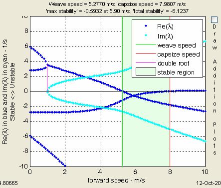
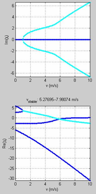
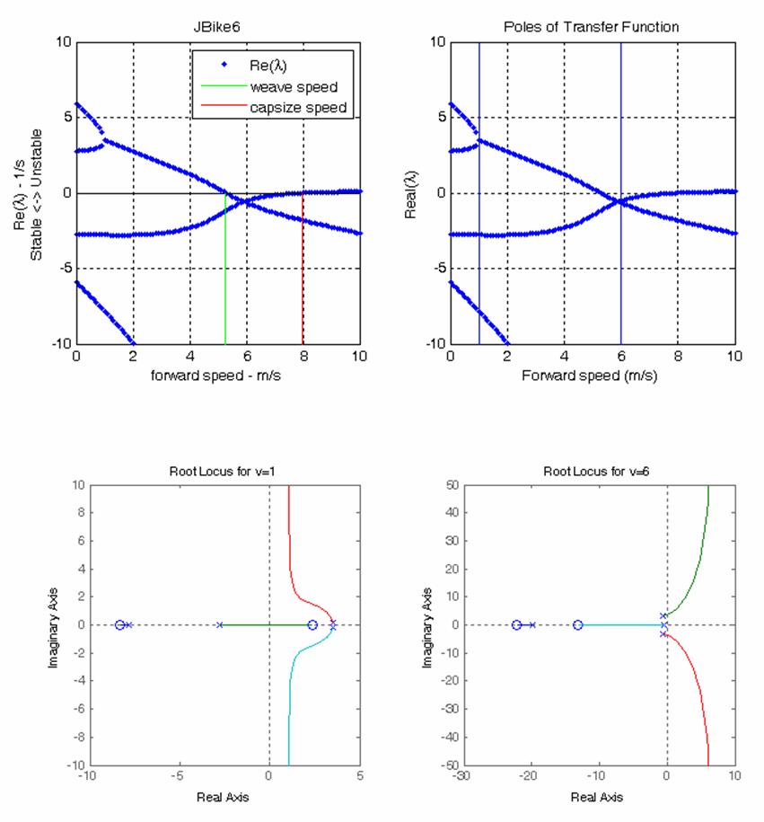
As an example consider, the eigenvalue plot for the Schwinn Crown.
 At forward speeds of 0 - 1 m/s: up to
emergence of complex conjugates
At forward speeds of 0 - 1 m/s: up to
emergence of complex conjugates
Large positive eigenvalues: very unstable. Two pos/neg pairs – both falling and uprighting. [Only one pair is seen for a simple inverted pendulum.] One pair corresponds to when the steering is turning toward the lean; the other when it is turning opposite to lean.
No imaginary parts of eigenvalues: not oscillating.
Just what you would expect from a bike standing still or nearly so. It will simply flop over.
At forward speeds of 1 - 5.2770 m/s: up to the weave speed
Positive eigenvalues, but decreasing in magnitude: unstable, but decreasingly so.
Eigenvalues with imaginary parts: oscillating with increasing frequency, and the rate of increase is rapid at first, but then slows.
The bike will weave back and forth one or more times before falling over.
At forward speeds of 5.2770 - 7.9807 m/s: the stable range: between the weave and capsize speeds
No positive eigenvalues, and increasingly negative: stable, and increasingly so.
Eigenvalues with imaginary parts: oscillating.
The bike will weave back and forth, less so each time, and eventually roll straight ahead, although not necessarily in the original direction.
At forward speeds of 7.9807 m/s and higher: above the stable range
Small positive eigenvalue: unstable
Eigenvalues with imaginary parts, but whose real component is much smaller than the positive eigenvalue: oscillations overwhelmed.
The bike slowly leans farther and farther to one side, without oscillation, until it finally falls over.
The transition between the behaviors in these speed ranges is as smooth and gradual as the curves in these plots suggest and can easily be seen in a numerical simulation with the same parameters.
That a bike loses stability at speeds higher than the capsize speed does not mean that it becomes harder to handle. This ‘capsize’ instability is very slow, on the order of seconds, and easy for a rider to compensate for. It is nothing like the ‘shimmy’ that some bikes exhibit at high speeds. That is an altogether different phenomenon usually based on frame flexibility (in bicycles) or tire flexibility (in motorcycles).
That JBike6 does not find a stable range of forward speeds for a particular bike configuration does not mean that in the real world it cannot be ridden or even that it would be hard to ride. Conversely, a stable range, no matter how big, does not mean that a bike will be easy to ride. Reality is more complicated than that. Two major factors that come into play on a real bike are that the rider is not really rigidly attached, and the rider may apply torques at the steering axis and between his mass and the frame. Other significant factors include friction between the wheels and the ground and at the steering axis.
A typical goal of analysis might be to adjust bike parameters and note how the ‘stable speed range’ is displaced or increased. Or, instead of uncontrolled STABILITY [negative eigenvalues], one might pay greater attention to BOUNDED GROWTH – a bike should be fairly rideable as long as no real part (or imaginary part with positive growth) exceeds about 4.0 in magnitude. In other words, one concept of a reasonable controllability criterion is that any eigenvalues in the right half plane should remain within a semicircle of radius 4.0.
Verification
The equations of motion for an idealized, uncontrolled bike used in JBike6 have been independently verified in a paper by A. L. Schwab, J. P. Meijaard, and J. M. Papadopoulos.
“The entries of the matrices of these equations form the basis for comparison. Three different kinds of methods to obtain the results are compared: pencil-and-paper [the equations used in JBike6], the numeric multibody dynamics program SPACAR, and the symbolic software system AutoSim. Because the results of the three methods are the same within the machine round-off error, we assume that the results are correct and can be used as a bicycle dynamics benchmark.”[3]
|
CTRL+A Draw axis lines on eigenvalue plot CTRL+B Draw coordinate axes on bike diagram CTRL+D Calculate and Draw Bike CTRL+E Draw additional eigenvalue plots in separate window CTRL+F Set ‘save bike’ directory… CTRL+G Draw grid lines on eigenvalue plot CTRL+H Help: Using JBike6… CTRL+I Draw imaginary parts of eigenvalues CTRL+J Interpolate double roots from calculated eigenvalues CTRL+K Set gravity constant… CTRL+L Draw legend on eigenvalue plot CTRL+M Use Styles menu styles in additional plots CTRL+N Save eigenvalues… CTRL+O About JBike6… CTRL+P Print Bike… CTRL+Q Quick Reference Guide… CTRL+R Draw double roots with vertical lines CTRL+S Save bike parameters CTRL+T Display status messages during calculations CTRL+U Print Setup… CTRL+V Draw weave speed with vertical line CTRL+X Exit CTRL+Y Save settings and styles when exiting CTRL+Z Draw capsize speed with vertical line |
About JBike6… CTRL+O Calculate and Draw Bike CTRL+D Display status messages during calculations CTRL+T Draw additional eigenvalue plots in separate window CTRL+E Draw axis lines on eigenvalue plot CTRL+A Draw capsize speed with vertical line CTRL+Z Draw coordinate axes on bike diagram CTRL+B Draw double roots with vertical lines CTRL+R Draw grid lines on eigenvalue plot CTRL+G Draw imaginary parts of eigenvalues CTRL+I Draw legend on eigenvalue plot CTRL+L Draw weave speed with vertical line CTRL+V Exit CTRL+X Interpolate double roots from calculated eigenvalues CTRL+J Help: Using JBike6… CTRL+H Print Bike… CTRL+P Print Setup… CTRL+U Quick Reference Guide … CTRL+Q Save bike parameters CTRL+S Save eigenvalues… CTRL+N Save settings and styles when exiting CTRL+Y Set gravity constant … CTRL+K Set ‘save bike’ directory… CTRL+F Use Styles menu styles in additional plots CTRL+M |
Note that changes in the ‘Plot Styles’ menu do not take effect until you calculate and draw the eigenvalues again.
Origin of JBike6
JBike6 is the successor of JBike5,
a Fortran program which was written by William Krauss and Jim Papadopoulos
around June 1988. Jim had worked closely with Scott Hand on his Master’s Thesis
at
JBike6 was created by Arend L.
Schwab of
Professor Andy Ruina of
|
Arend L. Schwab |
Jim
Papadopoulos |
Andy Ruina |
Andrew
Dressel |


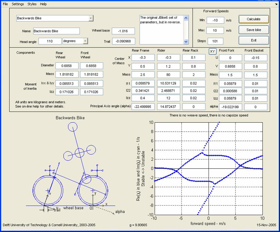
Rear steering
JBike6 provides a couple of options for examining the behavior of a bike with rear steering.
1. Simply specify a negative speed. This reveals that the eigenvalues are symmetrical about the x-axis exactly at the Re(λ )-axis, and that they have a wonderful inverse or mirror symmetry about the Re(λ )-axis.
2. Specify a backwards bike with negative wheelbase, trail, a head angle greater than 90°, etc.
There is not a hard line defined between front steering and rear steering. Instead there is just a continuous spectrum from most of the mass in the rear to most of the mass in the front, head angle positive to head angle negative, and trail positive to trial negative.
More on Gravity
The standard sea-level value of g
in physics tables is 9.80665 m/s2. It was set at the by the 3rd Conférence
générale des poids et mesures (General Conference on Weights and Measures) in
Little ‘g’ described above incorporates large ‘G’, the universal gravitational constant that expresses the gravitational attraction between two bodies, the radius of the earth, the mass of the earth, variations in the earth’s density, and the so-called ‘centrifugal force’ due to the rotation of the earth. It varies slightly from location to location on the surface of the earth.
The Physics Department at
More on Precision
MATLAB, the underlying mathematics software of JBike6, assigns numbers the data type double, which means that they are double-precision floating-point numbers that are 8 bytes (64 bits) in length. The internal representation is always the 8-byte floating-point representation provided by the particular computer hardware. On computers that use IEEE floating-point standard arithmetic (ANSI/IEEE Standard 754-1985 for Binary Floating-Point Arithmetic) (Intel Pentium and Celeron processors, for example), the resulting internal value is truncated to 53 bits. This is approximately 16 decimal digits.
The smallest magnitude is 4.9407e-324, and the largest is 1.7976e+308
You can see an example of the side effects due to the necessary conversion to base 2 and the finite nature of Standard 754 with these four operations in MATLAB:
a = 4 / 3
b = a - 1
c = 3 * b
e = 1 – c
They yield e = 2.220446049250313e-016, which is not the expected 0.0 from the 16th digit on.
You can read more about the IEEE standard 754 and MATLAB in ’Numerical Computing with MATLAB’ by Cleve Moler.
More on Parameters
Wheelbase = X of front wheel – X of rear wheel. JBike6 needs some nonzero fore-aft extent for things to make sense. Once again there is a dimensional scaling such that a shrunk bike behaves just like a full-sized bike, except over a shrunken speed range. And once again, while the limit of ‘zero’ for all lengths could be approached, it will only make sense if ratios are preserved. So you should think of fixing one dimension and varying the others.
Trail = X of steer axis – X of front wheel
Head angle: JBike6 produces identical results for values ±360, when using the uv-coordinate system, and ±180 when using the xy-coordinate system.
Wheel radius is irrelevant as long as the contact point is fixed and the ratio between inertia and radius (I/r) is fixed, while wheel-plus-assembly mass and cm are unchanged. JBike6 could actually use a much reduced input set, but uses traditional parameters for convenience and compatibility with other calculations.
Wheel Inertia: For a conventional wheel, Izz < mr2 and Izz < Ixx + Iyy must both be true. However, for a wheel geared to a slower-moving or faster-moving flywheel, which is located off the ground, these restrictions do not apply to Izz.
Mass: The eigenvalues remain unchanged by mass scaling, so there is nothing to learn by driving all masses to zero. You might as well fix one mass in the system and adjust all the others.
Inertia: JBike6 calculates the same result if you add or subtract 180° to the inertial principal axis angle or if you add 90° to the inertia principal axis angle and switch the values in I11 and I22. I11 does not need to be the larger value. Read more on Inertia Tensors at Wolfram Research and Wikipedia.
Conventionally, the y coordinate of every mass center should be positive. An exception might be a bike on an elevated path or walkway, with a ‘counterweight’ putting its cm below ground level.
Conventionally, a rider center of mass can not exist within the wheel radius, but it is possible with heavy saddlebags.
Conventionally, the overall center of mass should fall within the wheelbase or the bike will pitch over, unless wheels are magnetic or otherwise held to the ground.
More on Eigenvalues
“Eigenvalues are a special set of scalars associated with a linear system of equations (i.e., a matrix equation) that are sometimes also known as characteristic roots, proper values, or latent roots (Marcus and Minc 1988, p. 144).” Read further at MathWorld by Wolfram Research.
Here is another way to think of eigenvalues. First, consider an eigenfunction, the essence of which is 'solutions which evolve to remain self-similar'. Anything which evolves in such a fashion only changes magnitude, in proportion to current magnitude, i.e. exponential behavior. In a sense the determination of eigenfunctions is the key question, and the resulting eigenvalue can then be determined by plugging in the eigenfunction and noting the magnitude change [after one multiplication of a transition matrix, which could be based on an elapsed time interval].
In fact, you may consider the classical approach, given initially above, starting with eigenvalues, to be backwards. It is merely the trick that most quickly leads to finding the eigenfunctions, or indeed the eigenvalues after recognizing that the eigenvalues alone are needed to answer a stability question.
For the upright bike, any perturbation motion consists of time evolving lean and steer, with initial conditions on lean amount, lean rate, steer amount, and steer rate. The whole theory of eigenfunctions is that there is a complete set of special 'fundamental' motions (which evolve in self-similar fashion), and since the system is linear, any disturbance can be decomposed into fundamental motions, and its whole future evolution easily calculated when they are added together.
Any linear time-evolving, time-independent equations have the property that the sum of two solutions is also a solution. Therefore there is special value in looking for 'eigensolutions' - solutions that remain self-similar as they evolve, and hence evolve exponentially. Then any solution can be expressed as linear combinations of eigensolutions. For the purpose of studying stability, only the exponential growth, defined by the 'eigenvalues', is really needed.
So, eigenvalues are often found by relatively simple calculations, on the way to determining eigensolutions. For example when written in state space form, eigenvalues they are identified as 'expansion numbers' that make it possible to find self-similar (exponential) solutions, by the vanishing of a determinant (polynomial).
You can read more at Numerical Computing with MATLAB at The MathWorks
Another excellent on-line article about eigenvalues, eigenvectors, eigenspaces, and some of their applications can be found in Wikipedia.
 One
example of the utility of eigenvalues and their corresponding eigenvectors can
be seen in inertia
tensors. In general, it takes
6 numbers (Ixx, Iyy, Izz, Ixy,
Ixz, and Iyz) to describe the inertia
of a 3-dimensional object about its center of mass (cm). These are often arranged in a 3x3 matrix where 3 of the numbers
are repeated (Ixy, Ixz, and Iyz) to symmetrically fill out the 9 locations. It turns
out, though, that if the coordinate system used, with the origin always at the
center of gravity, is oriented properly, then only the 3 numbers along the
diagonal of the matrix (Ixx,
Iyy, Izz) are non-zero. In fact, these three numbers are the
eigenvalues of the 3x3 matrix, and the 3 axes of the necessary coordinate
system are the eigenvectors. This is how JBike6 only needs three numbers (Ixx, Iyy, Izz)
to describe the inertia of the parts of a bike when in general 6 numbers are
required. It also needs a Principal Axis Angle, the amount that the principal
axis is rotated from the horizontal, to complete the description
One
example of the utility of eigenvalues and their corresponding eigenvectors can
be seen in inertia
tensors. In general, it takes
6 numbers (Ixx, Iyy, Izz, Ixy,
Ixz, and Iyz) to describe the inertia
of a 3-dimensional object about its center of mass (cm). These are often arranged in a 3x3 matrix where 3 of the numbers
are repeated (Ixy, Ixz, and Iyz) to symmetrically fill out the 9 locations. It turns
out, though, that if the coordinate system used, with the origin always at the
center of gravity, is oriented properly, then only the 3 numbers along the
diagonal of the matrix (Ixx,
Iyy, Izz) are non-zero. In fact, these three numbers are the
eigenvalues of the 3x3 matrix, and the 3 axes of the necessary coordinate
system are the eigenvectors. This is how JBike6 only needs three numbers (Ixx, Iyy, Izz)
to describe the inertia of the parts of a bike when in general 6 numbers are
required. It also needs a Principal Axis Angle, the amount that the principal
axis is rotated from the horizontal, to complete the description
For more on how to generate eigenvalues and eigenvectors, see the next section.
More on Inertia Tensors
JBike6 provides only 3 spaces to specify the inertia tensors for the parts of a bike, whereas, in general, a 3-dimensional inertia tensor has 9 values usually arranged in a 3-by-3 symmetric matrix. In order to generate the 3 values that JBike6 requires, you can diagonalize the 3-by-3 matrix with MATLAB’s eig() function. The output of eig() is two matrices: the second is a diagonalized matrix with the desired 3 values (actually eigenvalues) along its diagonal, the first is a matrix with eigenvectors for columns
[V,D] = EIG(X);
I11 = D(1,1);
I22 = D(2,2);
Izz = D(3,3);
These eigenvectors are the axis necessary to express the inertia tensor with just 3 values. Because the eigenvectors are orthogonal and JBike6 requires symmetry about the x-y plane, you can simply use MATLAB’s atan() function to calculate the principal axis angle (alpha) that JBike6 needs from either the first or the second column of the second matrix returned by the eig() function:
Principal_axis_angle_in_degrees = atan(V(2,1),V(1,1))*180/pi();
For further discussion about eigenvalues, eigenvectors, and inertia tensors, see the last paragraph of the previous section.
More on the Bike Diagram
Any rigid body inertia tensor has three mutually perpendicular principal axes. It is possible to reproduce the inertia of a body by placing point masses out at the ends of three orthogonal rods. For the graphical representation, JBike6 divides a body’s mass into six equal lumps, each with 1/6 of the total mass. Then the rod half-lengths L1, L2 and Lz match the inertia tensor, deduced from the formulas
I11 = 2(m/6) * [L22 + Lz2]
I22 = 2(m/6) * [L12 + Lz2]
Izz = 2(m/6) * [L12 + L22]
Solved as (I11 + I22 – Izz) = 2(m/6) * [2Lz2], or Lz2 = (I11 + I22 – Izz) / (4m/6), etc.
Thus the mass moment of inertia about any one axis is large, if the two perpendicular rod lengths are large.
JBike6 indicates the size of the point masses by presenting them as modest size uniform-thickness disks, whose area indicates their mass. This is just a graphic convention; the mass-centric inertia of each disk is not considered when computing the overall moment of inertia. These are point masses, or masses pivoted at their centers so they don’t rotate, only translate.
Consider the disks to be made of steel [density taken as 7874 kg/m3], and with a thickness of two inches or 0.0508 m, radius R is defined from
M/6 = (density) * (volume) = (7874) * (πR2 * 0.0508) = 400 * πR2
The radial thickness of a wheel is shown in a consistent way – treating the rim as made of 2 inch thick steel, we write 400π(R02 – Ri2) = Mass of wheel, which permits us to solve for Ri.
More on the Equations of Motion
As JBike6 calculates the eigenvalues,
it displays in the MATLAB command
window, if you have the ‘display status messages during calculations’
option checked in the ‘Settings’ menu, the precise values of the equation
coefficients of the M, C, and K (the sum of K0 and
M = M0;
C = C1 .* v;
K = K0 +
With these equation coefficients, you can integrate to get the resulting bike motion.
Three cases are of special interest:
A. If the steer angle, as a function of lean angle from a control algorithm for example, is given, take the lean equation and put all steer terms on the right hand side. Then integrate to calculate bike lean.
B. If the steer torque, from a controller based on lean and steer angles for example, is given, you need the steer equation too. Then integrate for lean and steer angle.
C. If there is no steer control or torque, a special case of B, integrate both equations with moments equal to zero.
You can read about Integrating Ordinary Differential Equations (ODEs) at Mathworks.
More on Running JBike6 without the GUI
The included MATLAB file, JBike6Batch.m, gives another example of running JBike6 without the GUI. By calling the appropriate JBike6 modules, JBike6Batch.m calculates the weave and capsize speeds for a range of wheelbase, head angle, and trail values for a give bike. It then plots surfaces of these critical speed values against the parameters that generate them.
You can run JBike6Batch.m in MATLAB with any of the methods described above for running JBike6.m: from the MATLAB command-line or from the MATLAB editor.
By editing this MATLAB source file, you may specify the bike to analyze, the minimum values of wheelbase, head angle, and trial, and the number of different values of each to consider. JBike6Batch calculates all the required parameter values, the resulting critical speeds, and plots the surfaces as can be seen below. The top, solid surface is the capsize speed, and the lower, mesh surface is the weave speed.
As with the 4 additional eigenvalue plots, you can use all of MATLAB’s plot manipulation tools including zoom, pan, and 3D rotate.
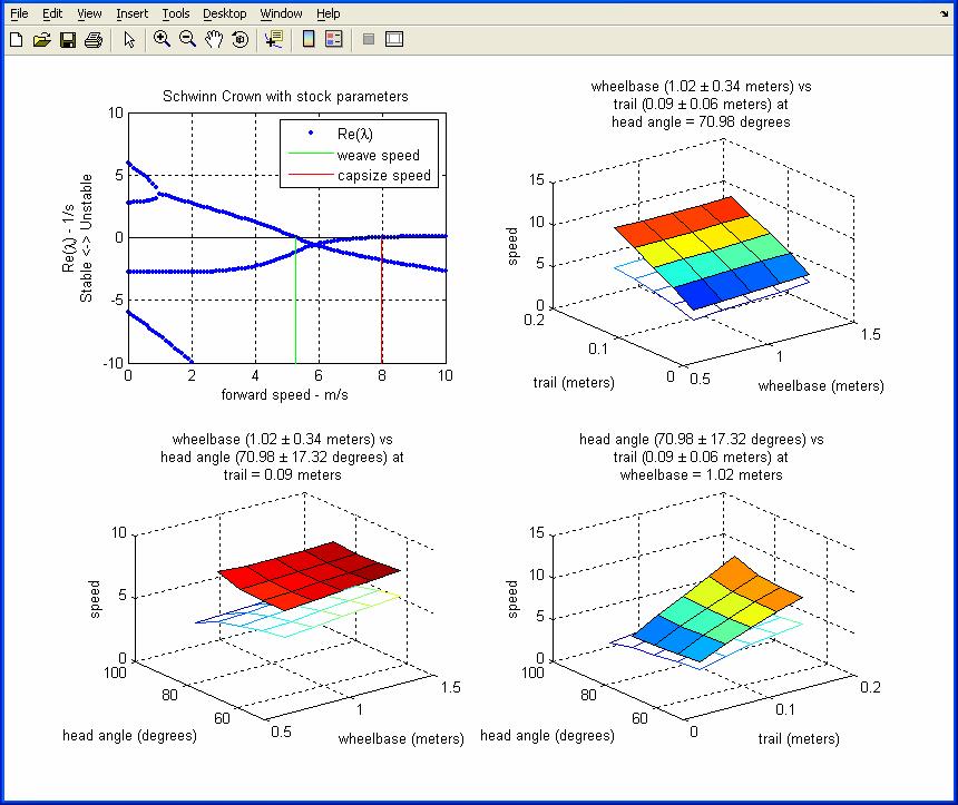
In this way, you can gain some idea of how varying key parameters of a bike will affect its hands-free stability.
Connecting JBike6 to MATLAB’s Control System Toolbox
The included MATLAB file, JBike6Control.m, gives another example of running JBike6 without the GUI. By calling the appropriate JBike6 modules, JBike6Control.m calculates the equations of motion and then arranges them as a transfer function appropriate for MATLAB’s Control System Toolbox. It then uses the pzmap() and rlocus() functions to generate a pole-zero map and a root-locus diagram.
Component Files
|
JBike6.m |
Main module, calls JBike6GUI.m |
|
JBike6GUI.m JBike6GUI.fig |
Graphical user interface, calls JBConfig, JBini, JBfig, JBmck, JBvcrit, JBeig, and JBref |
|
JBconfig.m |
Contains user savable parameters |
|
JBini.m |
Contains default parameters |
|
JBini_files |
Subdirectory with saved bike JBini*.m files |
|
JBfig.m |
Draws representation of bike in main window |
|
JBdrawcross.m |
Draw a cross to represent wheel hubs |
|
JBdrawinertia.m |
Draw the inertia ‘dumb bells’ |
|
JBdrawcircle.m |
Draw circles |
|
JBmck.m |
Calculates the linearized equations of motion |
|
JBaddb.m |
Adds the mass and inertia of rigid bodies into one body |
|
JBvcrit.m |
Calculates the weave and capsize speed |
|
JBcombint.m |
Combines two interval lists A and B into a new interval list C |
|
JBpolyint.m |
Makes an interval list A in x where the polynomial p(x) is positive. |
|
JBdoubleroots.m |
Calculates double root speed(s) analytically (uses Symbolic tool box) |
|
JBroots.m |
Calculates double root speed(s) by interpolation from eigenvalues |
|
JBeig.m |
Calculates the eigenvalues and eigenvectors |
|
JBrev.m |
Plots eigenvalues in main JBike6 window |
|
JBplot4.m |
Plots eigenvalues four ways in separate window |
|
JBhelp.htm |
Main help file |
|
JBhelp_files |
Subdirectory of support files: images |
|
JBQRef.htm |
Main quick reference file |
|
JBQRef_files |
Subdirectory of support files: images |
|
Readme.txt |
A few notes about how to get started with JBike6 |
|
License.txt |
Complete text of license agreement |
|
JBike6Batch.m |
A sample file demonstrating how to call the individual JBike6 components directly |
|
JBike6Control.m |
A sample file demonstrating how to plug JBike6 into MATLAB’s Control System Toolbox |
See the next section on JBike6 Architecture for more details
JBike6 Architecture
 The
architecture of JBike6 and its graphical user interface is designed to provide
both ease-of-use and versatility.
The
architecture of JBike6 and its graphical user interface is designed to provide
both ease-of-use and versatility.
Ease-of-use is provided by JBike6GUI.m and its companion file JBike6GUI.fig. These are created with MATLAB’s guide utility, and they create the entire user interface. By necessity, parameters are stored in MATLAB’s handle structure with the guidata() function so that they can be available to various call-back functions.
Versatility is provided the simple and flat structure of the mathematical modules. They contain MATLAB scripts that do not even need to pass parameters to each other. They simply define variables in MATLAB’s global space and access them as necessary. You can run them directly from the MATLAB command line and manipulate the variables as you go.
For example, you can load any set of bike parameters you want simply by running the appropriate JBini*.m file. Then, to calculate the linearized equations of motion, simply run JBmck.m. You can calculate the critical speeds with JBvcrit.m, the eigenvalues with JBeig.m, and then plot them with JBref.m. The calculated values of the critical speeds are contained in the vweave and vcapsize variables respectively.
See the previous section on the component files of JBike6 for more details.
Links
Bicycle Mechanics at Cornell University’s The Biorobotics and Locomotion Lab
MathWorld by Wolfram Research.
Numerical Computing with MATLAB by Cleve Moler
License
Use of JBike6 is licensed to you by the authors and limited by the license agreement. You agreed to its terms and conditions when you downloaded JBike6. A copy of the license agreement is included with the JBike6 program files in license.txt. You can also find a copy on the JBike6 website.
Read as ‘one-two coordinate system’. The coordinate system associated with each rigid body with its origin at the center of mass, and rotated, in this case about the z-axis, so that only 3 numbers, instead of the usual 6, are required to completely specify its inertia properties in 3D. In JBike6, you can specify the angle, called the principal axis angle, or alpha, that the 12-coordinate system is rotated from xy. The 1-axis is rotated counter-clock-wise from the x-axis, the horizontal, by alpha, and the 2-axis is rotated in the same direction from the y-axis, the vertical, by the same amount.
Alpha
The principal axis angle. The amount, for each body, that its 12-coordinate system (read as one-two, not twelve) is rotated about the z-axis from the xy-coordinate system.
ASCII text
American Standard Code for Information Interchange. A standard for assigning numerical values (7 binary digits) to the set of letters in the Roman alphabet and typographic characters. Read more at Wikipedia.
In this document, bicycle is the term used to represent a bike powered only by a rider, as opposed to a motorcycle. A bicycle is typically lighter than a motorcycle, especially relative to the rider, and usually has narrower tires.
In this document, bike is the term used to represent a device with two wheels connected to a frame and fork, one behind the other, and with a pivot so that one wheel may be turned with respect to the other for steering: either a bicycle or a motorcycle.
The forward speed at which capsize motion neither grows nor decays. This is represented by a vertical line on the eigenvalue plot.
Capsize motion is that motion in which the bike slowly leans and steers, without oscillation, farther and farther until it falls over.
At speeds above this capsize speed, the capsize motion will progress until the bike falls over. There may not be a capsize speed for a particular bike configuration. Odd designs have been found which have no finite capsize speed, and are stable at all speeds above the weave speed.
The point in space, not necessarily in or on the body, at which all the mass of the body may be considered to be concentrated for many mechanics calculations.
A means of interacting with an application through typed text strings, commands, as opposed to a GUI.
A mixture of real
and imaginary numbers, usually written a±bi,
where a is the real component, b is the imaginary
component, and ![]() . Complex numbers often arise as roots of equations.
. Complex numbers often arise as roots of equations.
The complex number associated with another complex number but with the opposite sign between the real and imaginary parts. The complex conjugate of a-bi is a+bi. Complex roots of equations usual come as complex conjugate pairs.
An origin and set of orthogonal axes, oriented according to the right-hand rule if in 3 dimension, that can be used to specify locations. JBike6 uses 3 different coordinate systems to completely specify a bike and its rider: xy, uv, and 12, all of which share a common z-axis.
Equations that share one or more variables so that they depend on each other: they cannot be solved independently. The equations of motion for a bike are a set of 2 coupled second-order ordinary differential equations.
Damped
harmonic oscillator equation
A common equation from classical
mechanics that describes the motion of a damped harmonic oscillator: a mass,
spring, dashpot. It is often written ![]() where x is a coordinate describing the
location of an object,
where x is a coordinate describing the
location of an object, ![]() is velocity of the
object: the first derivative with respect to time of coordinate x,
is velocity of the
object: the first derivative with respect to time of coordinate x, ![]() is the acceleration of the object: the second
derivate with respect to time of the coordinate x, m is the mass of the object, c
is the damping coefficient, and k is
the spring constant. The damping coefficient, c, describes how rapidly the dashpot damps the system, and the
spring constant, k, describes how
stiff the spring is.
is the acceleration of the object: the second
derivate with respect to time of the coordinate x, m is the mass of the object, c
is the damping coefficient, and k is
the spring constant. The damping coefficient, c, describes how rapidly the dashpot damps the system, and the
spring constant, k, describes how
stiff the spring is.
A matrix of the linearized equations of motion for a bike that multiplies the velocities, as does the damping term in classical damped harmonic oscillator equation.
Degrees
Angular unit of measure: equivalent to 0.0174533 radians. There are exactly 360° in a complete circle: 2π radians.
Degrees of freedom
The number of coordinates necessary to completely describe location and orientation. In 3-space, a 3-demensional body requires 6 coordinates (x, y, z, roll, pitch, and yaw) and so has 6 degrees of freedom. If the body is in motion, then it has 6 more degrees of freedom, the rate at which the first 6 change. For the analysis that JBike6 performs, the bike only has 2 degrees of freedom: lean angle of the rear frame, and steer angle of the front fork.
Equations of one or more variables and their derivatives.
Differential operator
A symbol that indicates that a variable is differentiated, often with respect to time. A superscript number to the right indicates how many differentiations.
Double roots
In JBike6, the forward speeds at which real eigenvalues come together and then split apart as complex conjugates. This signals the onset of oscillation. There may be more than one, and JBike6 indicates them by vertical lines on the eigenvalue plot.
Dumbbells
A technique JBike6 uses to graphically represent the rotational inertia properties of a body in the bike diagram. The mass of the body is distributed into 6 equal disks, drawn as circles and only 5 of which are visible in 2 dimensions, and placed on the end of 6 arms, only 4 of which appear in 2 dimensions. The arms are placed along the axes of the inertia tensor for the body. The length of the arms represents the resistance of the body to angular acceleration about the other two axes.
Eigenvalue Plot
In JBike6, a plot of the forward speed vs the corresponding eigenvalues of a particular bike configuration.
Eigenvalues are extensively covered above in two sections: Eigenvalues and More on Eigenvalues.
Equations that tell how a body, or system of bodies, move in time: usual second-order differential equations. In JBike6, the equations of motion for a bike are two, coupled, second-order differential equations.
A point at which a system is in balance: does not move. Equilibrium points may be stable or unstable. For a pendulum with a rigid arm, straight down is a stable equilibrium point, and straight up is an unstable equilibrium point: any perturbation will cause the pendulum to move exponentially away from that straight up position.
Euler’s equation
One of many amazing discoveries made by 18th century Swiss mathematician Leonhard Euler: exi = cos(x) + sin(x)i, where x is any real number, i is an imaginary number, and e is the base of natural logarithms. See further explanation and a proof at Drexel’s Math Forum.
A description of the motion of a system, especially with respect to equilibrium. Exponential growth is motion away from equilibrium, and exponential decay is motion towards equilibrium. In either case, the motion may be oscillatory. The expression ‘exponential’ is due to a commonly assumed form of the solution to the equation(s) of motion: x = eλt where x represents the position of the system, t is time, e is the base of the natural logarithms, and λ is a constant. If λ is positive, then x will grow for increasing values of t. If λ is negative, then x will decay for increasing values of t. If λ is zero, then x will remain constant: be in equilibrium. If λ is complex, then the motion will be oscillatory.
Usually the front part of a bike, that connects to the front wheel and the frame with revolute joints.
Forward speed is a variable in the equations of motion for a bike, and so the eigenvalues depend on forward speed. In JBike6, the units are meters-per-second, and you can specify a range of forward speeds to investigate. The word ‘speed’ is used, instead of ‘velocity’, a vector quantity, because the direction is not defined, other than that it is forwards instead of backwards.
Usually the rear part of a bike, where the rider sits, that connects to the rear wheel and the fork with revolute joints.
Frequency
The rate at which a motion repeats: measured in ‘cycles per second’ or ‘hertz’. Used to measure oscillatory motion.
Graphical User Interface (GUI)
Pronounced "gooey". A means of interacting with an application through a metaphor of direct manipulation of graphical objects, as opposed to a ‘command-line’ interface.
The gravitational constant extensively covered above in two sections: Gravity and More on Gravity.
Head angle
The angle that the bike head tube (steering axis) makes with the horizontal. By convention, positive angles are clockwise from the horizontal. A 90° head angle would be vertical. Common head angles for road bikes range from 70° to 75°.
The part of a bike frame in which the fork pivots.
Imaginary component
The part of a complex number which is an imaginary number.
A number which is a real number multiple of ![]() .
.
The property of matter that resists acceleration, either linear or rotational.
A description of a body’s inertia about its center of mass. Usually express in a 3x3 matrix of 9 values, 3 of which are repeated. If the 3 axes are oriented properly, then only 3 values are necessary.
Kilograms
Unit of mass used by JBike6: equivalent to 0.0685218 slugs. A kilogram weighs about 2.2 pounds at the surface of the earth.
An idealization use to simplify the equations of motion in JBike6’s bike model. It ignores the kinematics of leaning a bike with finite-radius tires.
The angle that the rear of a bike makes with the vertical. When the bike is straight upright, the lean angle is zero.
Equations that contain only ‘linear’ terms. Linear terms satisfy the following two properties: Additivity: f(x + y) = f(x) + f(y) and Homogeneity: f(αx) = αf(x) for all α. Examples of nonlinear terms include x2 and sin(x). Read more about linear and nonlinear systems.
Equations that have been
simplified to be linear. A common
‘linearization’ is that for small angles θ,
sin(θ) is approximately θ. The equation of motion for a simple pendulum, ![]() , may
be linearized in this way to
, may
be linearized in this way to ![]() which then has the
closed-form solution θ = C1e(g/ℓ)t + C2e(-g/ℓ)t.
which then has the
closed-form solution θ = C1e(g/ℓ)t + C2e(-g/ℓ)t.
The property of matter that gives it inertia and gravitational attraction.
A matrix of the linearized equations of motion for a bike that multiplies the accelerations, as does the mass term in classical damped harmonic oscillator equation. In JBike6 it consists of the mass and the inertia values of the particular bike configuration.
“MATLAB is a high-level language and interactive environment that enables you to perform computationally intensive tasks faster than with traditional programming languages.” Read more at The MathWorks web site.
A regular grid of values. Systems of linear equations and inertia tensors can both be expressed as matrices.
Meter
Unit of length used by JBike6: equivalent to 3.2808399 feet, 39.3700787 inches, 100 centimeters, 1000 millimeters, and 1.9102197 Royal Egyptian cubits.
Unit of speed used by JBike6: equivalent to 3.6 kilometers per hour, 2.2369363 miles per hour, mach 0.0029387, and 6,012.8727971 furlongs per fortnight.
In this document, motorcycle is the term used to represent a bike powered by some type of engine or motor, as opposed to a bicycle. A motorcycle is typically heavier than a bicycle, especially relative to the rider, and usually has wider tires.
Ordinary
Differential Equation (ODE)
Differential Equations distinguished from Partial Differential Equations (PDEs) which contain partial derivatives. The bike equations of motion that JBike6 uses are ODEs.
The location, part of a coordinate system, from which coordinates are measured.
Perpendicular to. At right-angles to. The x, y, and z axes that JBike6 uses are mutually orthogonal.
Motion which repeats itself. The swinging of a pendulum is oscillatory. For a bike, it is that motion in which the bike leans and steers back and forth.
A small change in the state of a body or system of bodies: often away from a point of equilibrium.
Precision
The number of digits used to perform a given computation. See the More on Precision section above.
In JBike6, the angle that 12-coordinate system (read as one-two, not twelve), used to express the rotational inertia of a body, is rotated from the xy-coordinate system.
Radians
Angular unit of measure: equivalent to 57.2957795 degrees. There are exactly 2π radians in a complete circle: 360°.
A number that is rational or irrational, not imaginary. Read more at Wikipedia.
Rear steering
A system in which the rear wheel pivots to steer a bike instead of the front wheel. There is not a hard line defined between front steering and rear steering. Instead there is just a continuous spectrum from most of the mass in the rear to most of the mass in the front, head angle positive to head angle negative, and trail positive to trial negative.
A connection between two bodies that constrains them to pivot with respect to each other about a common axis. Door hinges are common physical examples of revolute joints. In the bike model used by JBike6, the steering axis and the wheel hubs are revolute joints.
A convention used to keep track of the orientation of axes in 3 dimensions. Start with the fingers of the right hand oriented in the direction of the first axis (x); bend the fingers in the direction of the second axis (y); the extended thumb then points in the direction of the third axis (z).
An idealized entity that permits absolutely no internal motion: no flex, no twist, no vibration, etc. The concept of rigid bodies is useful for drastically simplifying the analysis of real-world objects.
Rolling without friction
A theoretical situation in which objects roll without any loss of energy due to friction. Ignores paradox of why they would roll at all instead of sliding. Useful for drastically simplifying the analysis of real-world objects.
Those values for which the
equation equals zero: where the curve of the equation crosses the x-axis. The
roots of a quadratic equation, ax2
+bx + c = 0, are given by ![]() .
.
If b2 is greater than 4ac then the roots are imaginary: a complex conjugate pair.
Second-order
differential equations
Differential equations involving variables and their second derivatives. The damped harmonic oscillator equation of motion is an example of a second-order differential equation.
Self-stable
In the case of a riderless bike, the property of returning to straight and upright (zero lean angle and zero steer angle) motion after a perturbation of either lean angle or steer angle.
The property of an object or system of objects in which it returns to a point of equilibrium after a perturbation.
State-space form
A way of expressing equations of motion in which the derivative of all the coordinates are found by multiplying all the coordinates by a matrix.
The angle, about the steer axis, between the front (fork and front wheel) and rear (frame and rear wheel) parts of a bike.
The imaginary line, usually through a head tube, about which both the rear frame and the front fork of bike rotate in order to steer.
Stiffness matrix
A matrix of the linearized equations of motion for a bike that multiplies the positions, as does the spring constant in classical damped harmonic oscillator equation.
The property of being the same on both sides of an axis or plane. The idealized bike that JBike6 uses is symmetrical about vertical plane down its middle: the left side and right side are mirror images of each other.
Tipping moment
The calculated tendency for a bicycle to tip forward around or over its front wheel. JBike6 calculates it by summing the products of each mass you specify with the distances, forward or behind, they are from the front wheel. If the result it positive, then JBike6 warns that a physical bike with these parameters would tip forward over the front wheel.
Tooltip
A small box containing helpful text that appears near a control of a GUI when you hover the mouse cursor over it.
Trail
The horizontal distance from the front hub (or ground contact point) to the point where the steering axis intersects the ground. By convention, positive trail is when the front wheel contact point is behind, toward the rear wheel, the steering axis intersect point.
The property of an object or system of objects in which it moves away from a point of equilibrium after a perturbation.
In JBike6, an optional coordinate system for expressing the location of the center of mass of the front fork and the front basket. Its origin is at the intersection of the steering axis and the ground plane and it is rotated so that what was its vertical axis is aligned with the steering axis.
Weave speed
The forward speed at which oscillatory motion neither grows nor decays. JBike6 represents this by a vertical line on the eigenvalue plot.
At speeds below this weave speed, the oscillations will grow until the bike falls over. There may not be a weave speed for a particular bike configuration
A conventional bike has a single nonzero speed interval of stability, and the weave speed is the lower boundary of this interval. Thus a bike that slows just below the weave speed, becomes unstable by weaving. But, if the weave speed is above the capsize speed, there probably is no stable interval.
Wheelbase
The horizontal distance between the hub (or ground contact point) of the front wheel and the rear wheel of a bike.
In JBike6, the coordinate system for expressing the location of the center of mass of the rear frame and the rear rack. Its origin is at the rear wheel ground-contact point, directly below the rear hub.
In JBike6, the coordinate axis that is ‘out of the plane’, that is orthogonal to the x and y axes, the u and v axes, and the 1 and 2 axes.
(to be columned and hyperlinked once finalized)