Simulation of the Simplest Walker

To ensure that our equations of motion for the Cornell Ranger are correct, we will now reduce the Cornell Ranger down to a simpler model. The simplest walker is a two dimensional bipedal passive walker that has point masses at the feet and hip and massless legs. By changing some of the parameters, we will be able to reduce the Cornell Ranger to the simplest walker and demonstrate that our dynamics are correct.

Figure 13. Simplest Walker Model

Reduction of the Cornell Ranger Model to the Simplest Walker

    To reduce the Cornell Ranger to the simplest walker, some of the parameters must be changed. The parameters that will be used are listed below.

    In addition, since the foot has a radius of zero, we can set two of the angles to be constant. We will lock  and  at pi.

    Lastly, we will allow the swing leg to pass through the ramp for near vertical stance leg angles. This will eliminate foot scuffing problems that occur in passive walkers. This problem which occurs in physical walkers can be overcome by adding knees, using stepping stones, or allowing the swing foot to lift up.

Fixed Points and Stability

    Before we continue on to create our simulation, we must first discuss the ideas of fixed points and stability. A step can be thought of as a stride function or Poincare map. This function takes a vector of the angles and angles rates at a particular point in the motion and returns the angles and rates at the next occurrence of that point. In our case, we will examine the point immediately after heelstrike. The result of the stride function can be found by integrating the equations of motion over one step.

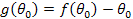
A period-one gait cycle exists if for a given set of initial conditions, the stride function returns the same conditions. That is, we are interested in the zeroes of as it is defined below.

    Additionally, we must check the stability of the cycles. We will do this by finding the eigenvalues of the Jacobian of the stride function, .  is constructed by evaluating the stride function with small perturbations to the components of the particular fixed point that is being evaluated. Small perturbations, , to the state vector, , at the start of a step will either grow or decay from the to the step by,

    If the eigenvalues of the Jacobian are within the unit circle, then sufficiently small perturbations will decay to zero and the system will return to the gait cycle. If any eigenvalues are outside the unit circle, perturbations along the corresponding eigenvector will grow and drive the gait cycle unstable. If any eigenvalues lie on the unit circle, the cycle is neutrally stable for small perturbations along the corresponding eigenvector and these perturbations will remain constant. We will use MATLAB to find the Jacobian and its eigenvalues.

Simplest Walker MATLAB Simulation

    We will now setup the simulation. Since we have reduced the Cornell Ranger to the simplest walker, we can re-use the equations of motion code that was derived for the Cornell Ranger. As and are locked, we drop the angular momentum balance equations about points  and  in figure 7. , , , , , and are required to find the necessary angles.

    A collision detection function must also be created. This function takes in the current time, positions, and parameters and determines if a collision has occurred. This function will be used with the integrator to stop ode113 from integrating when heelstrike occurs. The collision detection that was derived in the symbolic derivation is used. An exception is required to ignore foot scuffing.

function [gstop, isterminal,direction]=collision(t,z,GL_DIM)

M = GL_DIM(1); m = GL_DIM(2); c = GL_DIM(3);

I = GL_DIM(4); g = GL_DIM(5); l = GL_DIM(6);

w = GL_DIM(7); r = GL_DIM(8); d = GL_DIM(9);

gam = GL_DIM(10);

q1 = z(1); q2 = z(3);

q3 = z(5); q4 = z(7);

gstop = -l*cos(q1+q2)+d*cos(q1)+l*cos(-q3+q1+q2)-d*cos(q1+q2-q3-q4);

if (q3>-0.05) %no collision detection for foot scuffing

isterminal = 0;

else

isterminal=1; %Ode should terminate is conveyed by 1, if you put 0 it goes till the final time u specify

end

direction=-1; % The t_final can be approached by any direction is indicated by this

    Next, the main driver needs to be set up. First, the initial conditions vector and parameters are setup. The initial conditions vector only needs , , ,  and since  and  are constant. We must then find the fixed points for the walker. We will use the fsolve function to solve the fixed point equation, . fsolve will iterate upon the provided initial conditions until it finds the fixed points, zstar, to within the tolerance provided. Typically, Newton-Raphson methods are used to find the fixed points but the fsolve function works equally as well.

%%%% Root finding, Period one gait %%%%

options = optimset('TolFun',1e-13,'TolX',1e-13,'Display','off');

[zstar,fval,exitflag,output,jacob] = fsolve(@fixedpt,z0,options,GL_DIM);

if exitflag == 1

disp('Fixed points are');

zstar

else

error('Root finder not converged, change guess or change system parameters')

end

    The fixed point function calls the onestep function which integrates the equations of motion and uses the heelstrike equations over the number of steps specified . The fixed point function calls onestep for one step.

function zdiff=fixedpt(z0,GL_DIM)

zdiff=onestep(z0,GL_DIM)-z0;

    Next, we will find the stability of the found fixed points.

%%%% Stability, using linearised eigenvalue %%%

J=partialder(@onestep,zstar,GL_DIM);

disp('EigenValues for linearized map are');

eig(J)

    We will define a function partialder which will calculate the Jacobian of the Poincare map. The Jacobian is estimated using central difference method of approximating derivatives. Central difference is accurate to the perturbation size squared as opposed to the perturbation size for forward difference but requires a little less than twice the number of evaluations. We will use perturbations of size .

%===================================================================

function J=partialder(FUN,z,GL_DIM)

%===================================================================

pert=1e-5;

%%% Using central difference, accuracy quadratic %%%

for i=1:length(z)

ztemp1=z; ztemp2=z;

ztemp1(i)=ztemp1(i)+pert;

ztemp2(i)=ztemp2(i)-pert;

J(:,i)=(feval(FUN,ztemp1,GL_DIM)-feval(FUN,ztemp2,GL_DIM)) ;

end

J=J/(2*pert);

    We now setup the integration of the equations of motion. To do this we will create a function called onestep which will integrate the equations of motion over the specified number of steps. The function takes in the initial conditions, the parameters and the number of steps.

%===================================================================

function [z,t]=onestep(z0,GL_DIM,steps)

%===================================================================

M = GL_DIM(1); m = GL_DIM(2); c = GL_DIM(3);

I = GL_DIM(4); g = GL_DIM(5); l = GL_DIM(6);

w = GL_DIM(7); r = GL_DIM(8); d = GL_DIM(9);

gam = GL_DIM(10);

    We then must set up the function for calculating the fixed points. If no number of steps is specified, we will assume that we are trying to find the fixed points. In this case, we only want to return the final state of the robot.

flag = 1;

if nargin<2

error('need more inputs to onestep');

elseif nargin<3

flag = 0; %send only last state

steps = 1;

end

    Now, the motion can be integrated. In addition to setting the tolerances, an event will be set in the options. This event will call our collision function to detect for collisions while the equations of motion are being integrated. When a collision is detected, the integrator is stopped. When it is stopped, the heelstrike equations will be called using the final conditions from the integration of the single stance equations. The resulting state vector and time is then set to the initial conditions for integration of the next step. At the end of the steps, if flag is one, all of the positions and times are returned. If not, only the last positions are returned.

t0 = 0;

dt = 5;

t_ode = t0;

z_ode = z0;

for i=1:steps

options=odeset('abstol',2.25*1e-14,'reltol',2.25*1e-14,'events',@collision);

tspan = linspace(t0,t0+dt,1000);

[t_temp, z_temp, tfinal] = ode113(@ranger_ss_simplest,tspan,z0,options,GL_DIM);

zplus=heelstrike_ss_simplest(t_temp(end),z_temp(end,:),GL_DIM);

z0 = zplus;

t0 = t_temp(end);

%%% dont include the first point

t_ode = [t_ode; t_temp(2:end); t0];

z_ode = [z_ode; z_temp(2:end,:); z0];

end

z = [zplus(1:2) zplus(5:6)];

if flag==1

z=z_ode;

t=t_ode;

end

    Lastly, we animate the robot over the steps and create plots of the stance leg and swing leg angles.

Comparison to Results Using Simplest Walker Equations

    We can now check our simulation of the simplest walker based on the equations of motion of the Cornell Ranger by simulating the simplest walker using the equations of motion found in The Simplest Walking Model paper¹.

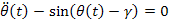
    We will use the reduced equations of motion.

Heelstrike:

For the reduced model of the Cornell Ranger, and .

Since we already have a walking simulation set up, we can simply replace the equations of motion in the appropriate sections.

In the single stance equations of motion function, we replace the  and  matrices with,

MM = [1 0; 1 -1];

RHS = [sin(q1-gam); cos(q1-gam)*sin(q3)-(u1^2)*sin(q3)];

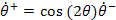
Additionally, in the heelstrike function, we replace the matrix calculation of the velocities with the following code.

u1 = cos(2*q1)*v1;

u2 = 0;

u3 = cos(2*q1)*(1-cos(2*q1))*v1;

u4 = 0;

Running the code reveals that the same fixed points are found and the resulting motion is the same. This result verifies our Ranger simulation.

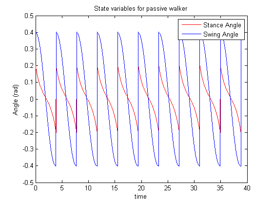
Figure 14. Plot of the Stance and Swing Angles for the Simplest Walker Paper Equations of Motion

Simplest Walker MATLAB File

1 The Simplest Walking Model Paper