Cornell Ranger Equations of Motion Derivation

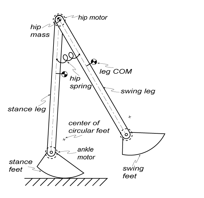
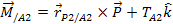
    To continue our exploration of dynamic simulations, we will symbolically derive the equations of motion for the Cornell Ranger. The model of the Cornell Ranger that will be used is depicted in figure 1 below. The model has one torsional spring at the hip.

Figure 6. Cornell Ranger Model and Terminology

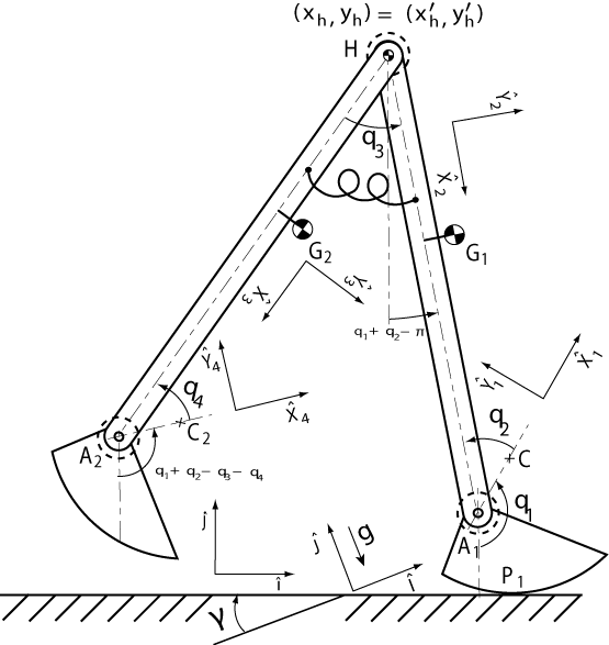
Figure 7. Cornell Ranger showing assumed coordinate systems and angles

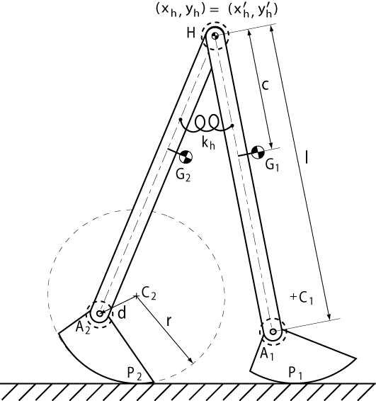
Figure 8. Cornell Ranger showing dimensions

Equations of Motion

    The dynamics of Cornell Ranger are much more complicated than that of the double pendulum. There is not one set of governing equations that can describe the dynamics of the walker for all time. Thusly, we must derive equations of motions for two distinct phases of motion, single stance and double stance, which depend on whether one or both feet are on the ground respectively. In addition, we must balance angular momentum before and after heelstrike. Heelstrike occurs the instant a foot collides with the ground.

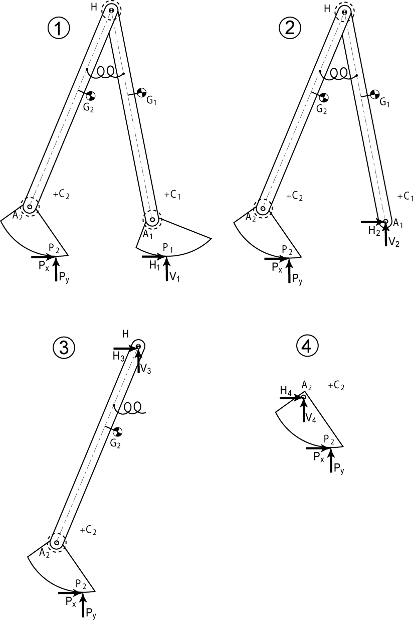
    Similarly to the double pendulum example, we will use the Newton-Euler method to solve for the equations of motion. We will first solve for the equations of motion for the single stance and double stance phases by perform four angular momentum balances, one for each of the free body diagrams below.

Figure 9. Free Body Diagrams of a) The entire walker, Angular Momentum balance about point b) The walker minus the front foot, Angular Momentum balance about point  c) The back leg, Angular Momentum balance about point  d) The back foot, Angular Momentum balance about point 

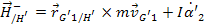
    From the four free body diagrams, we get,

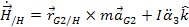
    where,

                                                                                                                             Masses of one leg and hip

                                                                                                                                     Inertia of one leg

                                                                                                                                    Inertia of motors

                                                                                                                                    Gravitational acceleration

                                                                                                                            Angular accelerations of the stance and swing leg

                                                                                                                                Acceleration of point 

                                                                                                                                Velocity of point 

                                                                                                                                 Hip motor torque

                                                                                                                               Hip spring torque

                                                                                                                          Torques at points  and 

                                                                                                                               External moment about point A

                                                                                                                                Rate of change of angular momentum about point A

                                                                                                                                   Force on the trailing leg in double stance

                                                                                                                                Position vector from point B to A

                                                                                                                                   Absolute angle made by stance foot and stance leg after and before heelstrike

                                                                                                                                   Relative angle between stance foot and stance leg after and before heelstrike

                                                                                                                                   Relative angle between legs; also hip angle after and before heelstrike

                                                                                                                                   Relative angle between swing foot and swing leg after and before heelstrike

                                                                                                                              Unit vectors along x, y and z axes

    For the single stance equations of motion, we solve for the angular accelerations while setting the trailing leg force, , equal to zero. For the double stance equations of motion, we solve for the angular accelerations while setting the trailing leg force, , equal to .

    In addition to these equations, we must also find two more equations from the two constraint equations that will enforce that the trailing leg rolls while the walker is in the double stance phase.  are found by writing the hip coordinate, , from the point of view of  while  are found by writing the hip coordinate from the point of view of .

    The two additional equations can be found by setting  and .

    We must now conserve angular momentum over heelstrike. We will look at the instances before and after heelstrike.

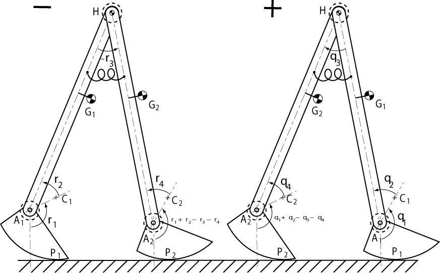
Figure 10. Cornell Ranger before and after heelstrike

Figure 11. Free Body Diagram before and after heelstrike, a) Entire walker b) Walker minus the forward foot

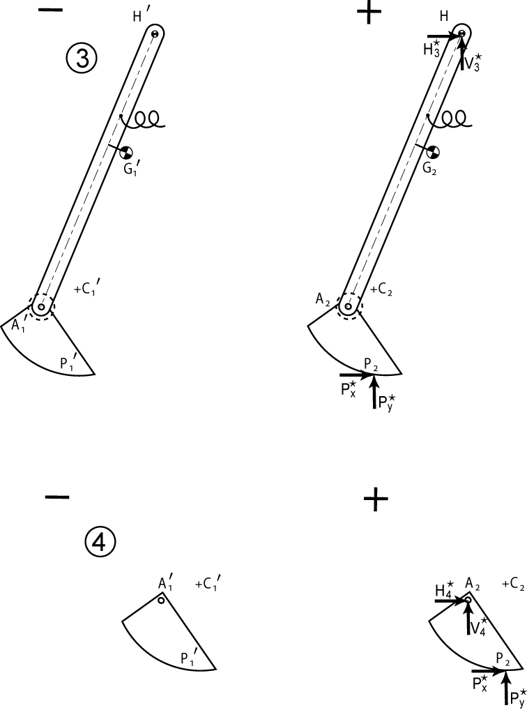
Figure 12. Free Body Diagrams before and after heelstrike, a) Back leg with foot b) Back foot

From the four free body diagrams, we get,

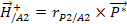
where,

                                                                                                                            Angular momentum about point 

                                                                                                                               Impulse on the trailing leg in double stance

    To transition into the single stance phase, the first three angular momentum equations are required and  should be set to zero. These equations need to be solved for the angular velocities.

    To transition into the double stance phase, all four equations are needed in addition to the first derivatives of the constraint equations,  and . Also,  should be set equal to  and the equations should be solved for the angular velocities.

Symbolic Derivation of the Equations of Motion in MATLAB

    Similarly to the previous example of a double pendulum, we start the symbolic derivation by defining the symbolic variables and parameters, defining the necessary reference frames, and defining the position vectors. We then set up the angular velocities and accelerations. We can now find the constraint equation and the linear velocities and accelerations.

q = [q1; q2; q3; q4];

u = [u1; u2; u3; u4];

ud = [ud1; ud2; ud3; ud4];

xH = l*sin(q1+q2)-d*sin(q1) - r*q1;

yH = -l*cos(q1+q2) + d*cos(q1) + r;

xG1 = xH+dot(r_H_G1,i);

yG1 = yH+dot(r_H_G1,j);

xG2 = xH+dot(r_H_G2,i);

yG2 = yH+dot(r_H_G2,j);

xH2 = -l*sin(q3-q1-q2)-d*sin(q1+q2-q3-q4)-r*(q1+q2-q3-q4);

yH2 = -l*cos(q3-q1-q2)+d*cos(q1+q2-q3-q4)+r;

xhdot1 = jacobian(xH,q)*u;

xhddot1 = jacobian(xhdot1,q)*u + jacobian(xhdot1,u)*ud;

yhdot1 = jacobian(yH,q)*u;

yhddot1 = jacobian(yhdot1,q)*u + jacobian(yhdot1,u)*ud;

xhdot2 = jacobian(xH2,q)*u;

xhddot2 = jacobian(xhdot2,q)*u + jacobian(xhdot2,u)*ud;

yhdot2 = jacobian(yH2,q)*u;

yhddot2 = jacobian(yhdot2,q)*u + jacobian(yhdot2,u)*ud;

v_H1 = xhdot1*i+yhdot1*j;

v_H2 = xhdot2*i+yhdot2*j; %velocties of hip assuming P1 and P2 is at rest resp.

vx_H = dot(v_H1,i);

vy_H =dot(v_H1,j);

a_H1 = xhddot1*i+yhddot1*j;

a_H2 = xhddot2*i+yhddot2*j; %accelerations of hip assuming P1 and P2 is at rest resp.

ax_H = dot(a_H1,i);

ay_H = dot(a_H1,j);

v_G1 = v_H1+cross(om2,r_H_G1);

v_G2 = v_H1+cross(om3,r_H_G2);

a_G1 = a_H1+cross(om2,cross(om2,r_H_G1))+cross(al2,r_H_G1);

a_G2 = a_H1+cross(om3,cross(om3,r_H_G2))+cross(al3,r_H_G2);

CD = yh - yhdash;

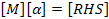
    Next, we will setup up the angular momentum balances and angular momentum terms. From these we will get the necessary equations for double stance, single stance and heelstrike. We will be solving for the equations in the form of,

    Additionally, we will derive the kinetic and potential energy. The next task is to have MATLAB create m-files containing the equations of motion for use in the simulation. The equations of motion for the Cornell Ranger are much more complicated than the double pendulum and it is much easier to have MATLAB automatically create the m-files. We will use the single stance file as an example.

    We will first create a file called single_stance.m using fopen with the 'w' permission. This allows us to create or writing to the file without regard to its current contents.

%%% Write single_stance.m %%%

fid=fopen( 'single_stance.m','w');

    We then have MATLAB write to the file using the fprintf command. This file will be setup in the same way the equations of motion file for the double pendulum was setup.

fprintf(fid, 'function zdot=single_stance(t,z,flag,GL_DIM) \n\n');

fprintf(fid, 'q1 = z(1); u1 = z(2); \n');

fprintf(fid, 'q2 = z(3); u2 = z(4); \n');

fprintf(fid, 'q3 = z(5); u3 = z(6); \n');

fprintf(fid, 'q4 = z(7); u4 = z(8); \n');

fprintf(fid, 'xh = z(10); vxh = z(11); \n');

fprintf(fid, 'yh = z(12); vyh = z(13); \n\n');

fprintf(fid, 'M = GL_DIM(1); m = GL_DIM(2); I = GL_DIM(3); \n');

fprintf(fid, 'l = GL_DIM(4); c = GL_DIM(5); w = GL_DIM(6); \n');

fprintf(fid, 'r = GL_DIM(7); d = GL_DIM(8); g = GL_DIM(9); \n');

fprintf(fid, 'gam = GL_DIM(10); \n\n');

fprintf(fid, 'Ta1 = 0; Th=0; Thip = 0; \n\n');

    Now we must write the  and  matrices. To do this, we will us the fprintf command but we must also convert the symbolic equation we have derived to characters to write to the file. In the following code, MATLAB replaces the %s with the second argument which contains the character version of the equation.

fprintf(fid,'M11 = %s; \n', char(simple(M_SS(1,1))) );

fprintf(fid,'M12 = %s; \n', char(simple(M_SS(1,2))) );

fprintf(fid,'M13 = %s; \n', char(simple(M_SS(1,3))) );

fprintf(fid,'\n');

fprintf(fid,'M21 = %s; \n', char(simple(M_SS(2,1))) );

fprintf(fid,'M22 = %s; \n', char(simple(M_SS(2,2))) );

fprintf(fid,'M23 = %s; \n', char(simple(M_SS(2,3))) );

fprintf(fid,'\n');

fprintf(fid,'M31 = %s; \n', char(simple(M_SS(3,1))) );

fprintf(fid,'M32 = %s; \n', char(simple(M_SS(3,2))) );

fprintf(fid,'M33 = %s; \n', char(simple(M_SS(3,3))) );

fprintf(fid,'\n');

fprintf(fid,'RHS1 = %s; \n', char(simple(RHS_SS(1))) );

fprintf(fid,'RHS2 = %s; \n', char(simple(RHS_SS(2))) );

fprintf(fid,'RHS3 = %s; \n', char(simple(RHS_SS(3))) );

fprintf(fid,'\n');

fprintf(fid,'MM = [M11 M12 M13; \n');

fprintf(fid,' M21 M22 M23; \n');

fprintf(fid,' M31 M32 M33]; \n\n');

fprintf(fid,'RHS = [RHS1; RHS2; RHS3]; \n\n');

fprintf(fid,'X = MM \\ RHS; \n\n');

fprintf(fid,'ud1 = X(1); \n');

fprintf(fid,'ud2 = X(2); \n');

fprintf(fid,'ud3 = X(3); \n');

fprintf(fid,'ud4 = 0; \n\n');

fprintf(fid,'DTE = %s; \n', char(simple(DTE)) );

fprintf(fid,'axh = %s; \n', char(simple(xhddot)) );

fprintf(fid,'ayh = %s; \n', char(simple(yhddot)) );

fprintf(fid,'\n');

fprintf(fid,'zdot = [u1 ud1 u2 ud2 u3 ud3 u4 ud4 ... \n');

fprintf(fid,' DTE vxh axh vyh ayh]''; \n');

fclose(fid);

Running this file yields files containing the equations of motion for single stance, double stance and heelstrike that are ready to use in a simulation.

Cornell Ranger Equations of Motion Derivation MATLAB File